Week 3 - Solving second order ODEs

Aim :-

• To write a program that solves the following ODE.
  
• Write a program in Python that will simulate the pendulum motion

##Conditions:-

• L=1 metre,
• m=1 kg,
• b=0.05.
• g=9.81 m/s2.
• Simulate the motion between 0-20 sec, for angular displacement=0,angular velocity=3 rad/sec at time t=0.

##Introduction:-

The motion of a simple pendulum is a basic classical example of simple harmonic motion, consisting of a small bob and a massless string.Movement of thependulum depends on the Newtons second law. When this law is written down,a second order Ordinary Differential Equation is formed that describes the position of the endof the pendulum w.r.t time.

##Procedure:

• Importing libraries

• Defining constant cofficients of equation
  

• Initial conditions:- At t = 0 , angular displacement for the pendulum is 0 and angular velocity is 3 rad per second.These conditions are stored in an array
  

• Time span :- A time array of 20 sec with 200 intervals is created upon which the ODE will be solved.
  

• Defining a differential function :-A function is created which represents the system of differential equation.

• Solving the ODEs :-

• Plotting the result

##Python Code-1 :-

#####Programme to save file for animation
import numpy as np
import math
from scipy.integrate import odeint
import matplotlib.pyplot as plt
# function
def model(T,t,b,length,gravity,mass):
    T1= T[0]
    T2 = T[1]
    dT1_dt = T2
    dT2_dt = -(b/mass)*T2 -(gravity/length)*math.sin(T1)
    dTh_dt = [dT1_dt, dT2_dt]
    return dTh_dt
# inputs
b = 0.05 # damping co-efficient
length = 1 # length of pendulum in m
gravity = 9.81 # gravity in m/s^2
mass = 1 # mass of ball in kg
# initial conditions
T_x = [0,3]
# time points
t = np.linspace(0,20,200)
# solve ode
T = odeint(model,T_x,t,args=(b,length,gravity,mass))
# plot
X = T[:,0]
ct = 1
for theta in X:
    x1 = 0;y1 = 0
    x2 = length*math.sin(theta)
    y2 = -(length*math.cos(theta))
    file = 'test%05d.png'%ct
    plt.figure()
    plt.plot([-1.5,1.5],[0,0],linewidth = 5)
    plt.plot([x1,x2],[y1,y2],linewidth = 4)
    plt.plot(x2,y2,'o',markersize =12)
    plt.xlim([-1.5,1.5])
    plt.ylim([-1.5,1.5])
    plt.savefig(file)
    ct = ct+1
    print(file)

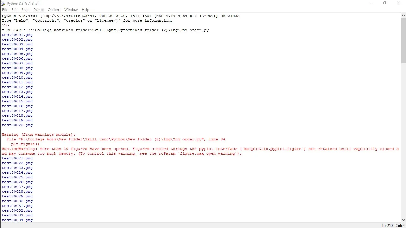
##output of code 1 :-

• 

##Python Code-2 :-

######Programme to plot displacement time graph

import math
import matplotlib.pyplot as plt
import numpy as np
from scipy.integrate import odeint
# function
def model(T,t,b,length,gravity,mass):
    T1= T[0]
    T2 = T[1]
    dT1_dt = T2
    dT2_dt = -(b/mass)*T2 -(gravity/length)*math.sin(T1)
    dTh_dt = [dT1_dt, dT2_dt]
    return dTh_dt
# inputs
b = 0.05 # damping co-efficient
length = 1 # length of pendulum in m
gravity = 9.81 # gravity in m/s^2
mass = 1 # mass of ball in kg
# initial conditions
T_x = [0,3]
# time points
t = np.linspace(0,20,200)
# solve ode
T = odeint(model,T_x,t,args=(b,length,gravity,mass))
# plot
plt.plot(t,T[:,0],'r-',label = 'Displacement')
plt.plot(t,T[:,1],'g--',label= 'Velocity')
plt.ylabel('plot')
plt.xlabel('time')
plt.legend()
plt.show()

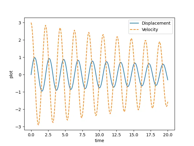
##output of code 2 :-

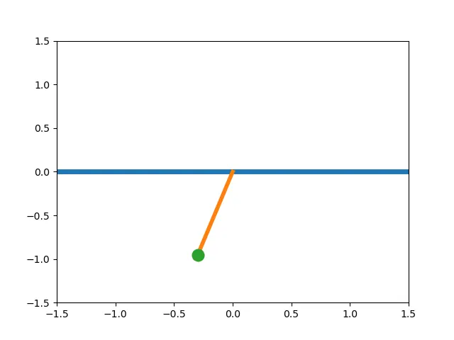
• Animation Of Pendulum Motion :-

##Conclusion : - The above graph shows the angular displacement and angular velocity and it changes over the time due to the effect of the damping, the values of reduce angular displacement and angular velocity with time as is clearly visible in above plot.