Solving second order ODEs by PYTHON

Objective

write a program that solves the following ODE. This ODE represents the equation of motion of a simple pendulum with damping.

Theory

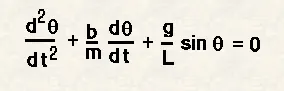
In the above equation,

g = gravity in m/s2,

L = length of the pendulum in m,

m = mass of the ball in kg,

b=damping coefficient.

^Code

import math
from scipy.integrate import odeint
import matplotlib.pyplot as plt 
import numpy as np



def mode1(theta,t,b,g,l,m):

	theta1=theta[0]
	theta2=theta[1]
	dtheta1_dt=theta2
	dtheta2_dt=-(b/m)*theta2-(g/l)*math.sin(theta1)
	dtheta_dt=[dtheta1_dt,dtheta2_dt]
	return dtheta_dt
	
	

b=0.05
g=9.81
l=1
m=1

#initial condition
theta_0=[0,3]

#time points
t=np.linspace(0,20,100)

	
#solve ODE
theta=odeint(mode1,theta_0,t,args=(b,g,l,m))

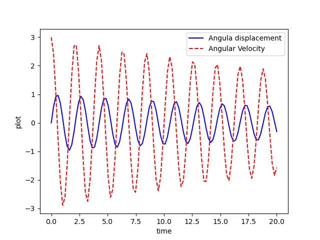
plt.plot(t,theta[:,0],'b-',label=r'Angula displacement')
plt.plot(t,theta[:,1],'r--',label=r'Angular Velocity')
plt.xlabel('time')
plt.ylabel('plot')
plt.legend(loc='best')
plt.show()

#Animation Step

ct=1
x0=0
y0=0
for i in range(len(t)):
	x1=x0+l*math.sin(theta[i,0])
	y1=y0-l*math.cos(theta[i,0])

	plt.figure()
	filename='pendulum'+str(ct)+'.png'
	ct=ct+1

	
	plt.hlines(0,-1,1)
	plt.plot([x0,x1],[y0,y1])
	plt.plot(x1,y1,marker='o',markersize='10')
	plt.xlim([-1.5,1.5])
	plt.ylim([-1.5,1.5])
	plt.savefig(filename)

Code Explanation

import math # required libraries are imported to the program
from scipy.integrate import odeint
import matplotlib.pyplot as plt
import numpy as np

def mode1(theta,t,b,g,l,m): #function definition

theta1=theta[0] #creating temporary variable theta1 to trace theta[0]
theta2=theta[1] #creating temporary variable theta2 to trace theta[1]
dtheta1_dt=theta2 #creating temporary variable dtheta1_dt to trace theta[2]
dtheta2_dt=-(b/m)*theta2-(g/l)*math.sin(theta1) #creating temporary variable dtheta2_dt as per formula
dtheta_dt=[dtheta1_dt,dtheta2_dt] #dtheta_dt saves as an array
return dtheta_dt #return dtheta_dt to the function

#input

b=0.05
g=9.81
l=1
m=1

#initial condition
theta_0=[0,3]

#time points
t=np.linspace(0,20,100)

#solve ODE
theta=odeint(mode1,theta_0,t,args=(b,g,l,m))

plt.plot(t,theta[:,0],'b-',label=r'Angula displacement')
plt.plot(t,theta[:,1],'r--',label=r'Angular Velocity')
plt.xlabel('time')
plt.ylabel('plot')
plt.legend(loc='best')
plt.show()

#Animation Step

ct=1 #set counter as 1
x0=0 #set initial point as origin
y0=0
for i in range(len(t)): #for loop from i to last point of length
x1=x0+l*math.sin(theta[i,0]) #creating traces by calculating end point
y1=y0-l*math.cos(theta[i,0])

plt.figure() #saving indivisual program
filename='pendulum'+str(ct)+'.png' #save indivisual figure as png format
ct=ct+1 #counter increament

plt.hlines(0,-1,1) #ploting figures
plt.plot([x0,x1],[y0,y1])
plt.plot(x1,y1,marker='o',markersize='10')
plt.xlim([-1.5,1.5])
plt.ylim([-1.5,1.5])
plt.savefig(filename)

all output files are stored in a folder and open cywin go to that folder then give command

magick *.png xx.gif

OUTPUT

Animation link

https://youtu.be/5KiYs5sVbaI