Simple pendulum animation by Solving second order ODEs

AIM:

To write a program in Python that will simulate the pendulum motion.

PROBLEM STATEMENT:

A ordinary differential equation (ODE) is a differential equation containing one or more functions of one independent variable and the derivatives of those functions. Ordinary, here, used to differentiate it from partial differential equation.

By solving the given ODE which refers to motion of simple pendulum we are going to find instantaneous angular displacements and respective angular velocities. By using them we are going to plot at all instances (of number we specified). At last we stich all plots to get smooth animation of simple pendulum in motion.

`(d^2 theta)/(d t^2)+b/m(d theta)/dt+g/Lsin(theta)=0`

let's assume

`theta_1=theta`

`frac{d\theta_1}{dt}=\theta_2`

`frac{d^2\theta_1}{dt^2}=(d\theta_2)/dt`

so

`{d\theta_2}/{dt}=-\frac{b}{m}\theta_2-\frac{g}{L}sin\theta_1`

Basic Trignometry (for position of string, bob)

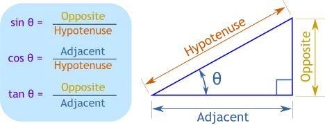
credit: https://www.mathsisfun.com/algebra/trigonometry.html

CODE WITH EXPLANATION:

1. Import modules (math-Mathematical functons like sin, cos etc; matplotlib.pyplot-plots; numpy-linspace; scipy-ode)
2. Define function funcdiff which returns solved ODE solution(angular displacemnent, angular velocity) as we discussed in problem statement.
3. Define inputs including b(damping coefficient) ,g(acceleration due to gravity), l(striing length), m (bob mass).
4. Define initial values of angular displacemnent, angular velocity in theta_0, here 0 and 3 respectively.
5. Define time array, here between 0 and 20 secs, with 150 instances (more instances, more execution time, better smoothness)
6. Solve the ODE function using odeint as per syntax below and store it in theta:
7. SYNTAX: parameter=odeint(function representing equation,initial values,time array, arguments/attributes of function)
8. Plot Angular veleocity and angular displacement vs time with necessary legend, axes label, title.
9. Define counting variable ct.
10. Define an array ang that stores angular diplacement of theta array.
11. Define origin x0 and y0.
12. Create for loop, inside it define x1 and y1 as per basic trignometry.
13. Plot:
14. Datum line
15. string
16. Bob position
17. Add title, legends, limit axes as per requiremnets
18. Store the generated image with naming appropriately using ct.
19. End of program

CODE with explanation in comments:

#SIMPLE PENDULUM USING 2nd ORDER ODE

import math
import matplotlib.pyplot as plt
import numpy as np
from scipy.integrate import odeint

#FUNCTION that returns d(theta)/dt
def funcdiff(theta,t,b,g,l,m):
	theta1=theta[0]
	theta2=theta[1]
	dtheta1_dt=theta2
	dtheta2_dt=-(b/m)*theta2-(g/l)*math.sin(theta1)
	dtheta_dt=[dtheta1_dt,dtheta2_dt]
	return dtheta_dt
#end of function

#inputs
#damping ratio
b=0.05
#acceleration due to gravity
g=9.81
#string length
l=1
#bob mass
m=1

#initial condition
theta_0=[0,3]

#time array, also notice no of instances, here 150
t=np.linspace(0,20,150 )

#solving ODE
#SYNTAX: parameter=odeint(function representing equation,initial values,time array, arguments/attributes of function)
theta=odeint(funcdiff,theta_0,t,args=(b,g,l,m)) 

#plotting begins
plt.plot(t,theta[:,0],'b-',label=r'$\frac{d\theta_1}{dt}=\theta2$')
plt.plot(t,theta[:,1],'r--',label=r'$\frac{d\theta_2}{dt}=-\frac{b}{m}\theta_2-\frac{g}{L}sin\theta_1$')
#labelling axes
plt.xlabel('Time')
plt.ylabel('Plot')
#legend location 
plt.legend(loc='best')
#saving figure
plt.savefig('AngDisp_AngVel_Time.png')
#displaying plot
plt.show()

#Angular displacements alone stored seperately
ang=theta[:,0]

#origin
x0=0
y0=0

#count
ct=0

#for loop to find bob position at each instant
for i in ang:
	x1=x0+math.sin(i)
	y1=-(y0+math.cos(i))
	ct=ct+1

	#plotting begins
	plt.figure()
	#Datum line
	plt.plot([-1,1],[0,0],linewidth=3)
	#string position
	plt.plot([x0,x1],[y0,y1])
	#BOB position
	plt.plot(x1,y1,'o',markersize=20)
	#limiting axes
	plt.xlim([-1.5,1.5])
	plt.ylim([-1.5,1.5])
	#Defining title
	plt.title("SIMPLE PENDULUM")
	#saving figure
	plt.savefig('%d_simple_pendulum.png'%ct)
	#plt.show()
#end of for loop
#end of program

RESULT:

Folder containing generated images:

Animation video link: https://youtu.be/6dUeOSI81G8

Angular displacement and Angular velocity vs Time

CONCLUSION:

From Angular displacement and Angular velocity vs Time graph it is clear that angular velocity and angular displacements reduces over time, this is because of air resistance and friction between string and its hinge point.

Also if we increase the, damping coefficient, the bob comes to rest sooner.

From the video it is clear that 20 secs is not enough for the bob to come to rest as damping coefficient is less, if we increase b, t will be less.