Week 3 - Solving second order ODEs
AIM: Write a program in Python that will simulate the pendulum motion.
INTRODUCTION:
In Engineering, ODE is used to describe the transient behavior of a system. A simple example is a pendulum
The way the pendulum moves depends on the Newton's second law. When this law is written down, we get a second-order Ordinary Differential Equation that describes the position of the "ball" w.r.t time.
Similarly, there are hundreds of ODEs that describe key phenomena and if you have the ability to solve these equations then you will be able to simulate any of these systems.
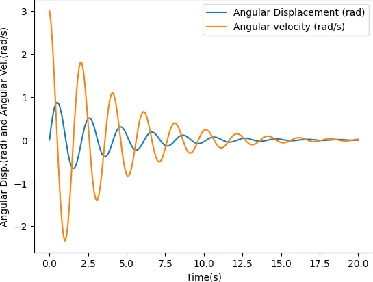
Your objective is to write a program that solves the following ODE. This ODE represents the equation of motion of a simple pendulum with damping
In the above equation,
g = gravity in m/s2,
L = length of the pendulum in m,
m = mass of the ball in kg,
b=damping coefficient.
Given that
L=1 metre,
m=1 kg,
b=0.05.
g=9.81 m/s2.
Simulate the motion between 0-20 sec
for angular displacement=0
angular velocity=3
rad/sec at time t=0.
PROGRAM:
# Importing libraries
import math
import numpy as np from scipy.integrate
import solve_ivp
import matplotlib.pyplot as plt
import os # Initial and end values
st = 0 # Start time (s)
et = 20 # End time (s)
ts = 0.1 # Time step (s)
g = 9.81 # Acceleration due to gravity (m/s^2)
L = 1 # Length of pendulum (m)
b = 0.5 # Damping factor (kg/s)
m = 1 # Mass of bob (kg)
# 1st order equations to solve in a function
def sim_pen_eq(t,theta):
dtheta2_dt = (-b/m)*theta[1] + (-g/L)*np.sin(theta[0])
dtheta1_dt = theta[1]
return [dtheta1_dt, dtheta2_dt]
# main
theta1_ini = 0 # Initial angular displacement (rad)
theta2_ini = 3 # Initial angular velocity (rad/s)
theta_ini = [theta1_ini, theta2_ini]
t_span = [st,et+ts]
t = np.arange(st,et+ts,ts)
sim_points = len(t)
l = np.arange(0,sim_points,1)
theta12 = solve_ivp(sim_pen_eq, t_span, theta_ini, t_eval = t)
theta1 = theta12.y[0,:]
theta2 = theta12.y[1,:]
plt.plot(t,theta1,label='Angular Displacement (rad)') plt.plot(t,theta2,label='Angular velocity (rad/s)')
plt.xlabel('Time(s)')
plt.ylabel('Angular Disp.(rad) and Angular Vel.(rad/s)')
plt.legend()
plt.show()
# Simulation
x = L*np.sin(theta1)
y = -L*np.cos(theta1)
for point in l:
plt.figure()
plt.plot(x[point],y[point],'bo',markersize=20)
plt.plot([0,x[point]], [0,y[point]])
plt.xlim(-L-0.5,L+0.5)
plt.ylim(-L-0.5,L+0.5)
plt.xlabel('Time(s)')
plt.ylabel('Angular Disp.(rad) and Angular Vel.(rad/s)')
filenumber = point
filenumber=format(filenumber,"05")
filename="image{}.png".format(filenumber)
plt.savefig(filename)
EXPLANATION:
The code will provide multiple frames of the pendulum's location corresponding to each time instant in the array 't' after solving the differential equation. Each of these frames or figures will be saved with the name format as 'image00000.png','image00001.png','image00002.png' and so on.
Then, the code will call the os and pass a comand line to the os to stich the images together to make a movie. Note that the definition of this comand line is in ffmpeg library. The figures and the movie will be saved in the same directory where the code file is saved.
youtube video link: https://youtu.be/7qD_kZK5w4s<iframe src="https://www.youtube.com/embed/7qD_kZK5w4s" allowfullscreen="allowfullscreen"></iframe>
CONCLUSION:
Hence we Write a program in Python that will simulate the pendulum motion for 0 to 20 sec.