Week 3 - Solving second order ODEs

The project involves the simulation of a simple pendulum ODE using Python programming.

AIM: To simulate the transient behavior of a simple pendulum and to create an animation of its motion

CODE:

import numpy as np
from scipy.integrate import odeint
import math
import matplotlib.pyplot as plt

def model(theta,t,b,g,l,m):
	theta1 = theta[0]
	theta2 = theta[1]
	dtheta1_dt = theta2 # first order ODE
	dtheta2_dt = -(b/m)*theta2 - (g/l)*math.sin(theta1) #first order ODE
	dtheta_dt = [dtheta1_dt, dtheta2_dt] #combining theta1 and theta2 to theta
	return dtheta_dt

b = 0.05 #damping coefficient
g = 9.81 # acceleration due to gravity m/s^2
l = 1 #length of the pendulum
m = 1 #in kgs

#initial conditions
theta_0 = [0,3]

#time points (time array)
t = np.linspace(0,20,200) # from t = 0 to 20 sec with 200 intervals

#solving ODE
theta = odeint(model,theta_0,t,args=(b,g,l,m)) #(system definition, initial condition, time, passing arguements)

#print(theta)
#plot results
plt.plot(t,theta[:,0],'b-', label=r'$\frac{d\theta_1}{dt}=\theta2$') #theta[:,0] represents displacement values
plt.plot(t,theta[:,1],'r--', label=r'$\frac{d\theta2}{dt}=-\frac{b}{m}\theta2-\frac{g}{L}sin\theta_1$') #theta[:,1] represents velocity values
plt.ylabel('Displacement')
plt.xlabel('time')
plt.legend(loc='best')
plt.show()

# To create Animation
ct = 1
x0 = 0 
y0 = 0

for i in theta[:,0]:
	x1=(1*math.sin(i))
	y1=(-1*math.cos(i))

	filename = str(ct)+'.png' #creating the filename and converting integer to string
	ct = ct+1 #for the generation of next count

	plt.figure()
	plt.plot([-1,1],[0,0],"red") #the roof for the pendulum
	plt.plot([x0,x1],[y0,y1],"black") #the length of the pendulum
	plt.plot(x1,y1,'o',markersize = '20') #the bob of the pendulum
	plt.xlim([-1.5,1.5]) #limiting the axis values
	plt.ylim([-1.5,1.0]) #limiting the axis values
	plt.savefig(filename) #Saving each frame
	plt.plot() #plotting the solution

A CONCISE DESCRIPTION OF THE CODE:

The code begins with the standard operation of importing the libraries. Followed by defining the function.

def model(theta,t,b,g,l,m):
theta1 = theta[0]
theta2 = theta[1]
dtheta1_dt = theta2 # first order ODE
dtheta2_dt = -(b/m)*theta2 - (g/l)*math.sin(theta1) #first order ODE
dtheta_dt = [dtheta1_dt, dtheta2_dt] #combining theta1 and theta2 to theta
return dtheta_dt

The function of the code is as follows:

The function is defined with regard to the input parameters and breaks down the second-order differential equation into 2 first-order differential equations. As it can be noticed from the program in the form of dtheta1_dt and dtheta2_dt and having it arranged in the final column matrix which provides the output.

The inputs for the code such as the damping coefficient 'b', accn due to gravity 'g' in m/s2, length of the pendulum'l' in m and the mass of the pendulum 'm' in kg are defined.

The initial conditions of angular displacement '0' and angular velocity of '3' rad/s.

The time array is defined between 0 to 20 sec with intervals of 200.

The ODE is solved using odeint and the function is defined with the along with the input parameters, time array and the initial condition. The function is run and the plot of varying velocity and displacement with respect to time can be observed below.

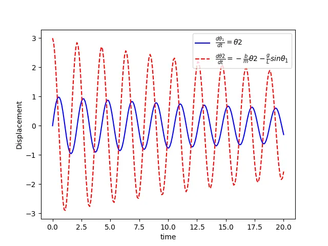
The plotting was carried out for the oscillations of the mass and the length using the plot command and providing appropriate size and color. Along with the definition of the axis that it is plotted in.

The ct command captures each frame for the loop of values and the images are then converted to a gif and uploaded on you tube the link to the animation is found below.

https://youtu.be/AZlsnv7mc8k