Week 3 - Solving second order ODEs

Aim: Write a program in Python that will simulate the pendulum motion

To write a program that solves the following ODE. This ODE represents the equation of motion of a simple pendulum with damping

In the above equation,

g = gravity in m/s2,

L = length of the pendulum in m,

m = mass of the ball in kg,

b=damping coefficient.

L=1 metre,

m=1 kg,

b=0.05.

g=9.81 m/s2.

Simulate the motion between 0-20 sec, for angular displacement=0,angular velocity=3 rad/sec at time t=0.

Solving the Equation:

`theta=theta1`

`(del^2theta1)/(delt^2)+b/m*(deltheta1)/(delt)+g/l*sin(theta1)=0`

`(deltheta1)/(delt)=theta2`

`(deltheta2)/(delt)+b/m*theta2+g/l*sintheta1=0`

Python Code:

"""
Program to solve second order differential equation
"""
import numpy as np
from scipy.integrate import odeint
import math
import matplotlib.pyplot as plt

# function that rteurns dz/dt

def model(theta,t,b,g,l,m):
    theta1 = theta[0]
    theta2 = theta[1]
    dtheta1_dt = theta2
    dtheta2_dt = -(b/m)*theta2-(g/l)*math.sin(theta1)
    dtheta_dt = [dtheta1_dt,dtheta2_dt]
    return dtheta_dt

b=0.01
g=9.81
l=1    
m=0.1   

# initial cond initial angle o deg and ang vel is 3 rad/s
theta_0 = [math.pi/2,0] 

# time points for 10 secs
t = np.linspace(0,10,150) 

# solve ode
theta = odeint(model,theta_0,t,args = (b,g,l,m))

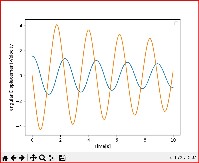
plt.plot(t,theta[:,0]) #plot first column and all rows
plt.plot(t,theta[:,1]) #plot second column and all rows
plt.xlabel('Time[s]')
plt.ylabel('angular Displacement-Velocity');
plt.legend(loc = 'best')
plt.show()

ct=1 # counter to capture each frame for the animation 

for i in theta[:,0]:
    # define initial coordinates of the pendulum rod about which it will rotate
   # print(i)
    x0=0
    y0=0
    # define final coordinates of the bob based on the result array
    x1=l*math.sin(i)
    y1=-l*math.cos(i)
    filename = str(ct) + '.png'
    ct=ct+1
    plt.figure()
    plt.plot([-0.5,0.5],[0,0],linewidth=5)
    plt.plot([x0,x1],[y0,y1],linewidth=2)
    plt.plot(x1,y1,'o',markersize=20)
    plt.xlim(-2,2)
    plt.ylim(-2,2) #define length of axis
    plt.grid()
    plt.title('Pendulum animation')
    plt.savefig(filename)

Code Explanation:

First we have to import all the relevant Library files like numpy, scipy, math and mathplotlib.

numpy is used to execute linspace function in order to generate an array

scipy to integrate the differential equation

math to solve the math functions like sin,cos etc

mathplotlib to plot the curves.

define the function model that defines the differential equation

Define the input variables

solve the differential equation using odeint function and plot the results.

Now plot the coordinates for the pendulum.

and generate animation

Results:

Youtube video link: https://youtu.be/6JSXDaLfVE8