Week 3 - Solving second order ODEs

Figure of Angular displacement and angular velocity with respect to time

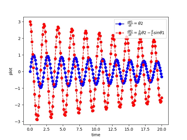
Code for ODE solution of Simple Pendulam

#simple pendulum

import math
import numpy as np
import matplotlib.pyplot as plt
from scipy.integrate import odeint

#input parameters
l=1 #meters
m=1 # kg
b=0.05
g=9.81 #m/s^2

"""
Equation of motion for simple pendulam with damping
d^2 theta/dt^2 + (b/m)(d theta/dt)+(g/l)sin theta = 0
theta = theta1
d theta1/dt = theta2
d theta2/dt = -(b/m)(d theta/dt)-(g/l)sin theta
"""

#function to find theta1 and theta2
def a (theta, t, b, m, g, l):
	theta1 = theta[0]
	theta2 = theta[1]
	d_theta1_dt = theta2
	d_theta2_dt = (-b/m)*(theta2)-(g/l)*math.sin(theta1)
	dtheta_dt = [d_theta1_dt, d_theta2_dt]
	return dtheta_dt

#Initial Conditions | angular displacement=0,angular velocity=3 rad/sec at time t=0
theta0 = [0,3]

#Boundary Condition
t=np.linspace(0,20,200)

#Solving for ODE
theta = odeint(a,theta0,t, args = (b, m, g, l))

# x0=np.empty(200); x0.fill(0)
# y0=np.empty(200); y0.fill(0)
x0=0
y0=0
ct = 1

theta_d = []
theta_d_cos=[]
theta_d_sin=[]
for i in theta[:,0]:
	theta_d_temp = i*180/math.pi
	theta_d_cos_temp = l*math.cos(i)

	theta_d_sin_temp = l*math.sin(i)
	theta_d_cos.append(-theta_d_cos_temp)
	theta_d_sin.append(theta_d_sin_temp)

	filename = str(ct) + '.png'
	ct=ct+1

	plt.figure()
	plt.plot((y0,theta_d_sin_temp),(x0,-theta_d_cos_temp), 'b-', marker = "o", markersize = 15)
	plt.ylim([-2,1])
	plt.xlim([-1,1])
	plt.savefig(filename)


	plt.show()

	theta_d = [theta_d_cos,theta_d_sin]
	#print (theta_d_temp)

#graph for displacement and velocity wrt time
plt.plot(t, theta[:,0],'b-', marker = "o", label=r'$\frac{d\theta1}{dt}=\theta2$')
plt.plot(t,theta[:,1],'r--', marker = "o", label=r'$\frac{d\theta2}{dt}=\frac{b}{m}\d\theta2-\frac{g}{L}sin\theta1$')
plt.ylabel('plot')
plt.xlabel('time')
plt.legend(loc='best')
plt.savefig('graph')
plt.show()