Week 3 - Solving second order ODEs

AIM: To solve Ordinary Differential Equation of Second order of Simple Pendulum using Python.

Objective:

To use Modules like numpy & scipy in the program.

To plot the graph of the positions and velocity of the simple pendulum.

Intoduction:

A pendulum is a weight suspended from a pivot so that it can swing freely.

When a pendulum is displaced sideways from its resting, equilibrium position, it is subject to a restoring force due to gravity that will accelerate it back toward the equilibrium position.

When released, the restoring force acting on the pendulum's mass causes it to oscillate about the equilibrium position, swinging back and forth.

The time for one complete cycle, a left swing and a right swing, is called the period.

The period depends on the length of the pendulum and also to a slight degree on the amplitude, the width of the pendulum's swing.

A simple pendulum consists of a mass m hanging from a string of length L and fixed at a pivot point P.

When displaced to an initial angle and released, the pendulum will swing back and forth with periodic motion.

By applying Newton's secont law for rotational systems, the equation of motion for the pendulum may be obtained

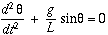
Program:

#Program to solve Odinary Differential Equations of Second order 
#Created by Abhishek Dhardwivedi
#Using Import to add libraries 
import numpy as np 
from scipy.integrate import odeint
import matplotlib.pyplot as plt 
import math

#Define a Function that returns dz/dt
def model(theta, t, b, g, l, m):
	theta1 = theta[0]
	theta2 = theta[1]
	dtheta1_dt = theta2
	dtheta2_dt = -(b/m)*theta2 - (g/l)*math.sin(theta1)
	dtheta_dt = [dtheta1_dt,dtheta2_dt]
	return dtheta_dt

#Inserting the values of the Coefficients appeard in the ODEquation of Simple Pendulum
b= 0.05
g=9.81
l=1
m=0.1

#initial Conditions
theta_0 =[math.pi/2,0]

#Time Inputs
t = np.linspace(0,20,150)

#Solving ODE
theta = odeint(model,theta_0,t, args=(b,g,l,m))

#Plot results
plt.plot(t,theta[:,0],'b-',label=r'$\frac{d\theta_1}{dt}=\theta2$')
plt.plot(t,theta[:,1],'r--',label=r'$\frac{d\theta_1}{dt}=-\frac{b}{m}\theta2-\frac{g}{L}sin\theta_1$')
plt.ylabel('Plot')
plt.xlabel('time')
plt.legend(loc='best')
plt.show()

Output:

Here, the Red Curves shows the oscillltion of the pendulum or the suspended mass.

Whereas, the Blue Curve shows the angular Velocity along the time period.