(ANSWER) -
A simple pendulum is a point mass suspended by a weightless and inextensible string fixed rigidly to support.
If the differential equation is 2 then it is called second order of ODE
The fundamental idea solving both analytically and computationally ,iffirst we have higher order we should break it into set of first order ode.
So,here from the calling function
function [dtheta_dt] = ode_f(t,theta,b,g,l,m)
theta1 = theta(1);
theta2 = theta(2);
dtheta1_dt = theta2;
dtheta2_dt = -(b/m)*theta2 - (g/l)*sin(theta1);
dtheta_dt = [dtheta1_dt;dtheta2_dt];
end
MAIN CODE -
close all
clear all
clc
% inputs given from above
% length of pendulum
l=1;
% mass of ball
m=1;
% Damping Coefficient
b=0.05;
% gravitational acceleration
g=9.81;
%initial conditions of displacement and velocity
theta_initial = [0;3];
%time points
t_span = linspace(0,10,600); %pendulum oscillates between 0-10seconds
%solve ODE
[t,result] = ode45(@(t,theta) ode_f(t,theta,b,g,l,m),t_span,theta_initial);
%plotting the graphs in one figure window and labelling
figure(1)
p1 = plot (t,result(:,1),'linewidth',3,'color','c');
xlabel('Time')
ylabel('Theta velocity')
title('BETWEEN VELOCITY,THETA VS Time')
%hold the figure for further plotting
hold on
p2 = plot(t,result(:,2),'linewidth',3,'color','b');
xlabel('Time')
ylabel('theta velocity')
title('BETWEEN VELOCITY,THETA VS Time')
legend([p1(1),p2(1)],'angular displacement','angular velocity')
%pendulum simulation using ode
theta = result(:,1);
% value to counter
ct=1;
% for loop to oscillate the pendulum
for i=1:length(result)
THETA = result(i,1);
%initial boundary conditon of pendulum
x0=0;
y0=0;
%Defining values x and y coordinates foe end destination of pendulum
x1= l*sin(THETA);
y1=-l*cos(THETA)
%creating figure for animation of pendulum
figure(2)
hold on
plot([x0 x1],[y0 y1],'linewidth',4);
plot(x1,y1,'.','markersize',50,'color','r','markerfacecolor',[0.2 0.2 0.2]);
plot(x0,y0,'-','markersize',30,'color','r','markerfacecolor',[0.2 0.2 0.2]);
axis([-2 2 -2 2]);
%foe each intervals
pause(0.002);
%getting the figure and storing in the form of array M(induvidual frame
%saved in array called M)
M(ct)=getframe(gcf);
%increment in counter fig
ct=ct+1;
%clearing the graphic images
clf()
end
%CREATING MOVIE
movie(M)
videofile = VideoWriter('simple_pendulum','uncompressed AVI');
open(videofile)
writeVideo(videofile,M)
close(videofile)
PLOTS OUTPUT -
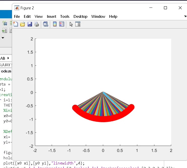
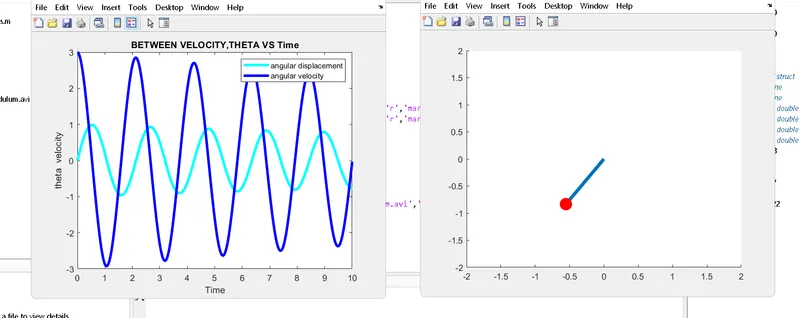
EXPLAINATION OF CODE -
Starting with commands.
Given inputs.
Here when solving ode there are 2 first order ode’s i.e initialdisplacement and initial velocity.
Here t_span is time which goes from 0 to 10 for 600 values.
Here from calling function we have
(ode45(@(t,theta) ode_f(t,theta,b,g,l,m),t_span,theta_initial
here ode_45 is inbuilt function in matlab here the main inputs are t and theta as these only the dependent and independent variables .
defining remaining input parameters with initial conditions with corresponding to time)
plotting both in different windows label and title the plot.
now,
for pendulum simulation ,for oscillation of pendulum we create the ‘for loop’ is generated and initial boundary coditions with x and y coordinates inputed and plotting the graph and fitting it into frame and created animated movie.
FINALLY ANIMATED MOVIE PLOT -
https://drive.google.com/file/d/1XEy9D1l4D29xwZNu7e7QH18oJfBTZZ3-/view?usp=sharing
ERRORS -
Common errors happen some like this later observed and corrected it all.
