Week 3 - Solving second order ODEs

write a program that solves the following ODE.

This ODE represents the equation of motion of a simple pendulum with damping

In the above equation,

g = gravity in m/s2,

L = length of the pendulum in m,

m = mass of the ball in kg,

b=damping coefficient.

Input :

L=1 metre,

m=1 kg,

b=0.05.

g=9.81 m/s2.

Simulate the motion between 0-20 sec, for angular displacement=0,angular velocity=3 rad/sec at time t=0.

Procedure :

• Initially we are importing the "Matplotlib.pyplot", "math", "scipy" and "numpy" library for the calculations.
• Scipy library provides us a the equation of second Order Differential Equation to solve the theta values.
• Then just inputing the given parameters g,b,l and m to calculate the other parameters.
• Using the function calling command we are going to call theta values.
• Then using "numpy" library command to provide steps in a time.
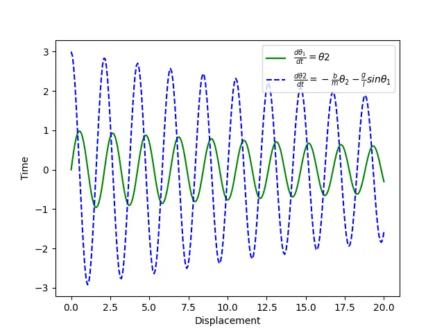
• Plotting Time against Displacement graph.
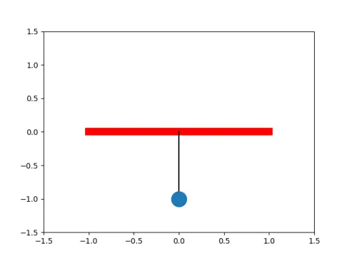
• For the motion of the simple pendulum, first mention the co-ordinates of the pendulum from the starting (x0, y0) and ending (x1, y1).
• String and counter command is used to give different png names and save all the png files.
• Then for Animation we use some othe Software for creating Animation.

Program :

# second order ODE
import numpy as np

from scipy.integrate import odeint
import matplotlib.pyplot as plt
import math


# calling function
def model(theta, t, b, g, l, m):
    theta1 = theta[0]
    theta2 = theta[1]
    dtheta1_dt = theta2
    dtheta2_dt = -(b / m) * theta2 - (g / l) * math.sin(theta1)
    dtheta_dt = [dtheta1_dt, dtheta2_dt]
    return dtheta_dt


# input parameters
b = 0.05
g = 9.81
l = 1
m = 1

# Initial condition
theta_0 = [0, 3]  # Angular displacement and angular velocity

# Time point
t = np.linspace(0, 20, 250)  # 0 to 20 sec motion

# Solve ODE
theta = odeint(model, theta_0, t, args=(b, g, l, m))

# Point results
plt.plot(t, theta[:, 0], 'g-', label=r'$\frac {d\theta_1}{dt}=\theta2$')
plt.plot(t, theta[:, 1], 'b--', label=r'$\frac {d\theta2}{dt}= -\frac{b}{m}\theta_2 -\frac{g}{l}sin\theta_1$')
plt.xlabel('Displacement')
plt.ylabel('Time')
plt.legend(loc='best')
plt.show()

# Animation of simple pendulum

# Fixed point at the wall
x0 = 0
y0 = 0

ct = 1
for ang in theta[:, 0]:  # angle
    x1 = l * math.sin(ang)
    y1 = -l * math.cos(ang)

    filename = str(ct) + '.png'
    ct = ct + 1

    plt.figure()
    plt.plot([-1, 1], [0, 0], 'red', linewidth=10)
    plt.plot([x0, x1], [y0, y1], 'black')
    plt.plot(x1, y1, 'o', markersize=20)
    plt.xlim(-1.5, 1.5)
    plt.ylim(-1.5, 1.5)
    plt.savefig(filename)

Plotting :

Animation :

Video :

Link - Simple Pendulum