Week 3 - Solving second order ODEs

clear all
close all
clc

%Given data

b=0.5;
m=1;
l=1;
g=9.81;

%Intitial Conditions

theta_0=[0;3];
t_span=linspace(0,10,1000);

% ODE function solving
[t,results]=ode45(@(t,theta)ode_function(t,theta,b,m,l,g),t_span,theta_0);

%Plotting graph

figure(1)
hold on
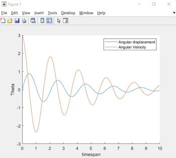
plot(t,results(:,1))
plot(t,results(:,2))

xlabel('timespan')
ylabel('Theta')
legend('Angular displacement','Angular Velocity')
% Pendulum Animation

% Introducing counter

ct=1;
for i=1:length(t)
x0=0;
y0=0;
x1=-l*sin(results(i,1));
y1=-l*cos(results(i,1));

figure(2)

plot([x0,x1],[y0,y1],'linewidth',2)
hold on
line([-1 1],[0 0])
plot(x1,y1,'.','MarkerSize',50)
hold off

axis([-1 1 -1 1])
M(ct)=getframe(gcf);
ct=ct+1;

end

% Creating Movie file
movie(M)
videofile=VideoWriter('D:\Skill lync\sample programs\Second order ODE\Pendulum_ODE.avi','uncoompressed AVI');
open(videfile)
writeVideo(videofile,M)
close(videfile)
% ODE Function declaration
function [result_matrix]=ode_function(t,theta,b,m,l,g)
theta1=theta(1);
theta2=theta(2);
dtheta1=theta2;
dtheta2=(-b/m)*theta2-(g/l)*sin(theta1);
result_matrix=[dtheta1;dtheta2];
end

Output:

Plot:

Animation Link: https://youtu.be/erakBNVw_EM