Week 3 - Solving second order ODEs

Aim:-
To solve an ordinary differential equation (ODE)and use the calculated information to animate
the motion of the pendulum via MatLab.

Introduction:-
Pendulums have many applications and were utilized often before the digital age. They are used
in clocks and metronomes due to the regularity of their period, in wrecking balls and playground
swings, due to their simple way of building up andkeeping energy.
A simple pendulum consists of a point mass suspended on a string or wire that has negligible
mass. If the pendulum weight or bob is pulled to arelatively small angle from the vertical and let go,
it will swing back and forth at a regular period andfrequency.

Code Explanation:-

% A function program which will be called in the main programe to solve the ODE
function [dtheta_dt] = ode_func(t, theta, b,g,l,m)
thetal= theta(1)
theta2= theta(2)
dthetal dt = theta2
dtheta2 dt- (b/m)*theta2 - (g/1)*sin(theta1)
dtheta_dt = [dthetal_dt; dtheta2_dt]
end
A function is a group of statements that togetherperform a task. In MATLAB, functions are defined in
separate files. The name of the file and of thefunction should be the same. Functions operate
on variables within their own workspace, which isalso called the local workspace, separate from
the workspace you access at the MATLABcommand prompt which is called the base workspace.
Function handles are simple to function codesthat can be created without using the regular
function definition using the keywords "function' and 'end'. They do not require any separate 'm'
files or not needed to be declared separately below/above the main code. Function handles
are directly declared in the main code itself andalso accessible from any point in that particular
code, i.e they are localized to a particularconditional. The declaration of a function handleis very similar to that of a function declaration. It can be distinguished by the means of '@' symbol
before your value/expression allocation. The syntax for creating a function handle is. A function
was defined in order to establish a relation between all the given input values,

code

clear all
close all
clc

b=0.05;
g=9.81;
l=1;
m=0.1;

% initial conditions

theta_0 =[0;5]

% time points

t_span = linspace(0,20,600)

% solve ODE

[t,results] = ode45(@(t,theta) ode_func(t,theta,b,g,l,m),t_span,theta_0);

plot(t,results(:,1))
hold on 
plot(t,results(:,2))
ylabel('plot')
xlabel('time')

% for loop

ct =1;
for i =1:length(results(:,1))
x_start =0
y_start =0
x_end  = l*sin(results(i,l))
y_end = -l*cos(results(i,l))


% ploting the animation

figure(2)
plot ([-1 1], [0 0], 'LineWidth',5)
hold on 
plot ([x_start x_end], [y_start y_end],'LineWidth',3)
hold on

plot (x_end ,y_end,'o','MarkerSize',20,'MarkerFaceColor','r')
title('animation of transient behaviour of the pendulum')
axis([-1.5 1.5 -1.5 1])
pause (0.03)
hold off

M(ct)=getframe(gcf)
ct=ct+1

end

% animation of the pendulum

movie(M)
videofile=VideoWriter('pendulum animation.avi','Uncompressed AVI')
open(videofile)
writeVideo(videofile,M)
close(videofile)

code explanation

Before writing the code, it's important to start with

clear all, close all and cc commands since
Clear all - removes data from the workspace,
freeing up system memory
Close all- deletes the current figure or the
specified figure
clc - clears all input and output from the
Command Window display, giving you a "clean
screen
Next step is to define the inputs and variables. The damping coefficient, gravity, length of the spring
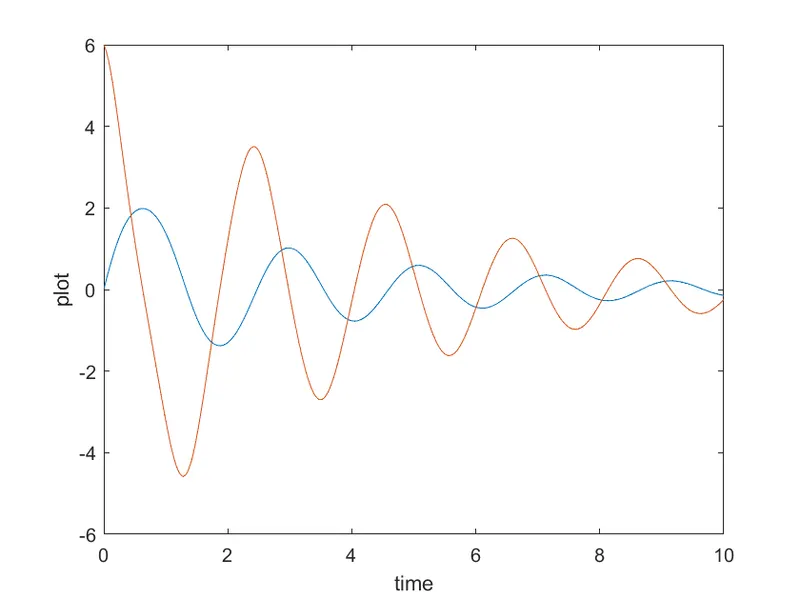
and mass of the bob have all been defined. Next step is to define the initial conditions, the angular displacement and angular velocity have been defined. Timespan has also been defined. Next step is to solve the ODE, Ode45 was used, it is a function in Matlab that solves ordinary or partial differential equations using a numerical method. The numerical method in question here is the 4th
order Runge Kutta method. The function ode45 takes 3 inputs. The 3 inputs are the function to be
integrated, the time span and the initial conditions. It, results means that the results that have been calculated with respect to time. After calculating the results, a graph has to be plotted, the graph contained two plots. One for angular displacement with respect to time and one for angular velocity with respect for time. The legend for the graph and the axis labels have been defined.

The second part of the code is to establish a for loop, A for loop is a repetition control structure
that allows you to efficiently write a loop that needs to execute a specific number of times. a
counter loop was added before the For loop. the start and endpoints for y and y-axis have been
defined. The loop is used where all the values of timespan are assigned to a variable "' one at a
time. The coordinates of [ xo xl y0 yij and their corresponding relations are
entered to form a 'string' of the pendulum. Markersize command was used to form the bob of
the pendulum. A pause command was used for pausing the command for a certain time, for this project a pause of 0.03 s was used. The M command was used to capture the current frame every time the for loop runs. The final step of the loop is to add a +1 to the ct variable; this will increment the frame every time the for loop run. End command was used for the plot and for the for loop to stop both from running.
The final step of the code is to create a movie of the animation of the robotic arm, so the movie command was used. The VideoWriter command was used to assign the video format, for this project .avi was used as the format. The open command was used to open the video. writevideo command was used to write the video with plot frames. Finally, the close command was used to close the video file.

ANIMATION VIDEO LINK :- https://drive.google.com/file/d/1cGJLIo2Cd9QsjcaOE1bTmEgwqiIumZK6/view?usp=sharing