Week 3 - Solving second order ODEs

Objective

To solve the second ODE using a pendulum represented as a spring-mass damped system.

Introduction

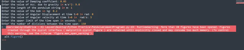
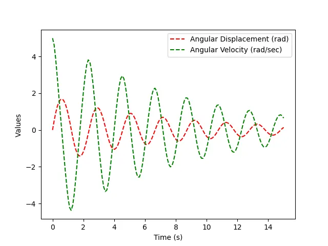
The code is written to solve the equations with any kind of input and the program will be successful, please bear in mind to keep the limits of the graph accordingly. Even though the program has slightly different inputs than the requested inputs this is only done to see a variation in inputs. The initial idea was to use imageio module to make an animation of the pictures that are drawn from the program. However, the command would not read the files, hence the module is not used. There are no errors with the program however there is a warning since the module matplotlib is used to plot. The code is given an explanation at every point. and is shown below.

# Program to solve the second order ODE with Simple Pendulum as a case
import math
import matplotlib.pyplot as plt
import numpy as np
import scipy as sp
import imageio as io
from scipy.integrate import odeint


#define the function 

def pendulum(theta,t,b,g,l,m): #function to give two seperate sets of values to the ODE solver 
	theta1 = theta[0]
	theta2 = theta[1]
	dtheta1 = theta2
	dtheta2 = -(theta2*(b/m))-(math.sin(theta1)*(g/l))
	dtheta = [dtheta1,dtheta2] # dtheta is a solution array with first column as displacement and second as velocty 
	return dtheta
	

# Defination of inputs 
b = float(input('Enter the value of Damping coeffcient: '))  #Manual control to change the damping 
g = float(input('Enter the value of Acc. due to gravity in m/s^2: ')) #Manual control over gravity 
l = float(input('Enter the length of the pendulum string in m: ')) #Manual control over length 
m = float(input('Enter the value of the bob in kg: ')) #Manual control over mass

# Intial conditions 
A_D = float(input('Enter the value of Angular Displacement at time t=0 in rad: ')) #Manual control over dispacement 
A_V = float(input('Enter the value of Angular velocity at time t=0 in  rad/s: ')) #Manual control over velocity 

theta_not=[]
theta_not.append(A_D)
theta_not.append(A_V)

dt = int(input('Enter the upper limit of the time span in seconds: ')) #Manual control over time in seconds
d = int(input('Enter the number of divisions between the time span: ')) # Manual control over fineness of division 

t = np.linspace(0,dt,d)

theta = odeint(pendulum,theta_not,t, args= (b,g,l,m)) #funtion call

plt.figure()
plt.plot(t,theta[:,0], 'r--', label = 'Angular Displacement (rad)') 
plt.plot(t,theta[:,1], 'g--', label = 'Angular Velocity (rad/sec)')
plt.legend(loc= 'best')
plt.xlabel('Time (s)')
plt.ylabel('Values ')
plt.show()



Teta1 = []

for D_Teta1 in theta[:,0]:
	Teta1.append(D_Teta1)

count =1

for D_Teta2 in Teta1:
	x0 = 0;
	y0 = 0;

	x1 = l*math.sin(D_Teta2)
	y1 = -l*math.cos(D_Teta2)

	file = 'Osilations%05d.png' %count
	count = count+1;

	plt.figure()
	plt.plot([-0.2,0.2],[0,0])
	plt.plot([x0,x1],[y0,y1])
	plt.plot(x1,y1,'-o')
	plt.xlim([-1.5,1.5])
	plt.ylim([-1.5,1])
	plt.title('Osilations of Pendulum')
	plt.savefig(file)
	

Results are given below