Week 3 - Solving second order ODEs
In Engineering, ODE is used to describe the transient behavior of a system. A simple example is a pendulum
whare
g = gravity in m/s2,
L = length of the pendulum in m,
m = mass of the ball in kg,
b=damping coefficient
L=1 metre,
m=1 kg,
b=0.05.
g=9.81 m/s2.
Simulateing the motion between 0-20 sec, for angular displacement=0,angular velocity=3 rad/sec at time t=0.
The code
function [dtheta_dt] = ode_func(t, theta, b, g, l,m)

theta1 = theta(1);
theta2 = theta(2);
dthetal_dt = theta2;
dtheta2_dt = -(b/m) *theta2 - (g/l)*sin(theta1);
dtheta_dt = [dthetal_dt; dtheta2_dt];
end
clear all
close all
clc
%given values
b=0.05;
g=9.81;
l=1;
m=1;
theta0=[0;3];
time = linspace(0,20,500);
[t, b] = ode45 (@(t,theta) ode_func(t, theta, b, g,l,m),time,theta0);
figure(1)
plot(t,[b(:,1) b(:,2)])
xlabel('Time in sec')
ylabel('Angular Displacement & Angular velocity(rad/sec)')
legend('Angular Displacement', 'Angular Velocity (rad/sec)')
hold on
axis([0 22 -3 3])
%Simulation of Pendulum
theta = b(:,1);
c = 1 ;
for i = 1:length(theta)
% theta1= theta(i);
x0=1;
y0=1;
x1 = 1-l*sin(theta(i));
y1 = 1-l*cos(theta(i));
figure(2)
plot([0 2],[1 1], 'linewidth',5, 'color', 'k');
hold on
% plot([x0 x1], [y0 y1], 'color', 'b', 'linewidth',3);
% hold on
plot([1 x1],[1 y1],[x1 x1],[y1 y1],'o', 'markers', 20, 'color', 'r', 'markerfacecolor', 'r');
hold off
grid on
axis ([0 2 -1 1.5])
pause(0.03)
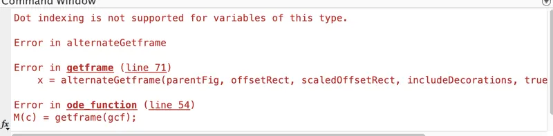
M(c) = getframe(gcf);
c= c +1;
end
movie (M)
videofile = VideoWriter('pendulum.avi', 'uncompressed AVI');
open(videofile)
writeVideo(videofile,M)
close(videofile)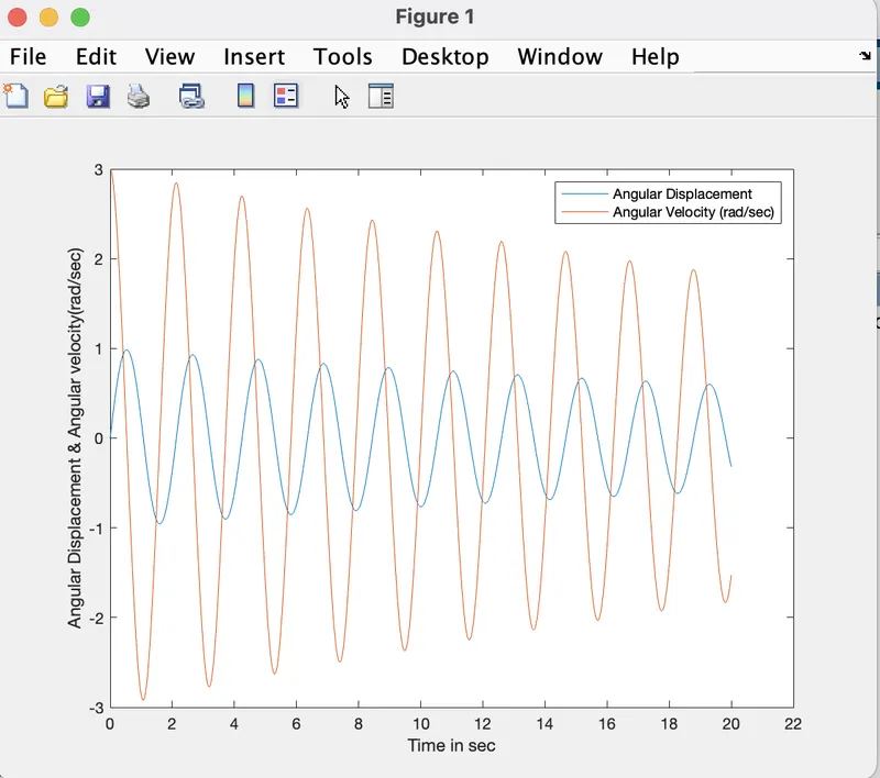
youtube link