Week 3 - Solving second order ODEs

b =0.2;
g = 9.81;
l = 1;
m = 0.1;

%intial condition
theta_0 = [0,3];

%time point
t_span = linspace(0,10,100);

% slove ode
[t,results] = ode45(@(t,theta) ode_func(t,theta,b,g,l,m),t_span,theta_0);

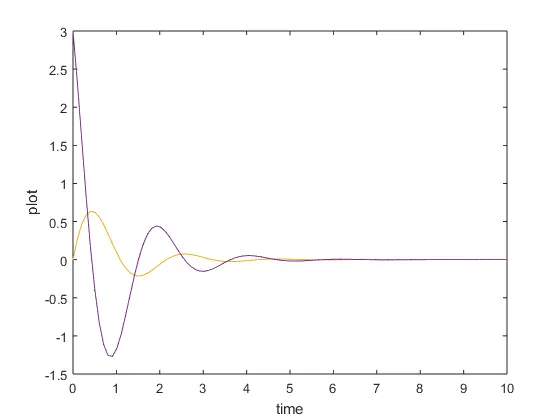
plot(t,results(:,1))
hold on
plot(t,results(:,2))
ylabel('plot')
xlabel('time')

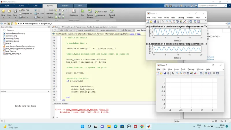
%% the program to solve an ODE IVP OF DAMPAD pedulum motion
%specifying system condition:

m = 1;
l = 1;
b = 0.05;
g = 9.81;

%specifying the inline function for pendulum ode:

f = @(t,x) [x(2);-(b/m)*x(2)-(g/l)*sin(x(1))];

%spcifying the intial condition at t=0

ini_cond = [0;3];

%spcifying the time range:

t = [0 20];

%solving the ODE:

[t,x] = ode45(f,t,ini_cond);
%% plotting the solution;

figure(1);

subplot(2,1,1);
plot(t,x(:,1));
grid on;

xlabel ('Time(s)');
ylabel ('angle(rad)');
title('Damped ocillation of a pendulum:angular displacement vs Time plot');

subplot(2,1,2);
plot(t,x(:,2));
grid on;

xlabel ('Time(s)');
ylabel ('angle(rad)');
title('Damped ocillation of a pendulum:angular displacement vs Time plot');

%% Animation of the damped pendulum in matalab

% Origin:
O = [0 0];
% aspect ratio of the plot:

figure(2);

axis (gca,'equal');

% plotting limits:

axis ([-1.2 1.2 -1.2 0.2]);
grid on;

% loop for animation:

for i = 1:length(t)
%specifying the point of the ball:

P = [l*sin(x(i,1))-l*cos(x(i,1))];
% circle in origin

% pendulum line :

Pendulum = line([O(1) P(1)],[O(2) P(2)]);

%specifying pedulum bomb and hinge point as circles:

hinge_point = viscircles(0,0.02);
bob_point = viscircles (P, 0.05);

%time interval to update the plot:

pause (0.0001);

%updaring the plot:
if i<length(t)

delete (pendulum);
delete (bob_point);
delete (hinge_point);

end
end