Week 3 - Solving second order ODEs

1. INTRODUCTION:-

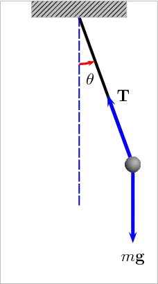
The pendulum is a body or mass suspended from a fixed point so that it can swing back and forth under the infiuence of gravity. Pendulums are used to regulate the movement of clocks because the interval of time for each complete oscilation, called the period, is constant. The period depends on the length of the pendulum and also to a slight degree on the amplitude, the width of the pendulums swing .

2.AIM:-

To solve the second- order ode function using Matilab which depicts the motion of the pendulum and to create an animation of the same.

3.OBJECTIVE

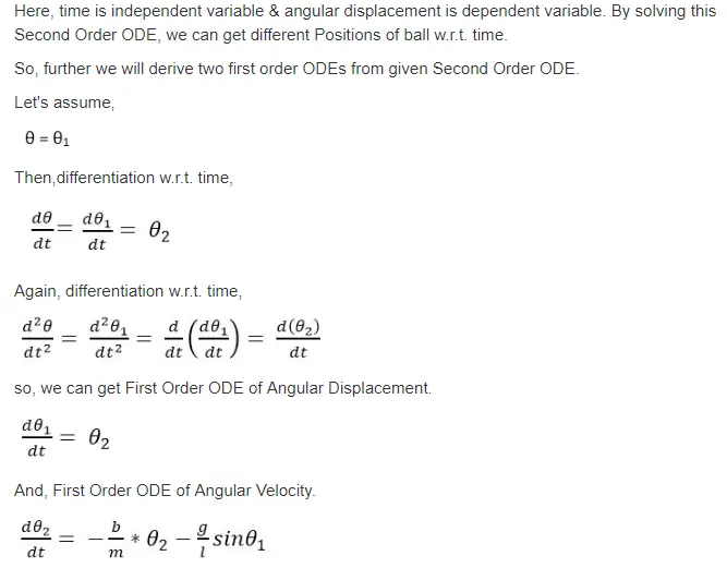
To write a program that solves the folliowing ODE. This ODE represents the equation of motion of a simple pendulum with damping

In the above equation

g= gravity in m/s2

L= longth of the pendulum in m,

m=mass of the ballin kg

b=damping coefficient.

FIXED PARAMETERS

Length (l)=1 metre,

Mass (m) =1 kg

Damping coiefficient (b) =0.05.

Acceleration due to gravity (g) =9.81 m/s2

For Time period = 0-20 sec

Angular displacement= 0, Angular velocity=3 rad/sec at time t=0.

4. PROGRAM

clear vars
close all
clc
  b= 0.01;      % damping co-efficient
  g = 9.81 ;   
  l = 1;        % length 
  m = 0.1;      % mass

  % initiAL CONDITION 
theta_0= [0;3];            %initial conditions defined to be theta equals zero(degree) and velocity equals 3 (m/s^2)

% TIME POINTS 
time_span = linspace(0,20,500);

 % SOLVE ODE
[t,results] = ode45(@(t,theta) ODE_FUNC(t,theta,b,g,l,m),time_span,theta_0);   % [t,results] is the column matrix we get from ODE_FUNC

% ode 45 is a ode solver program in matlab 
% ode45(@(t,theta) signiefies that the ode is a function of 't' and 'theta'
% ODE_FUNC(t,theta,b,g,l,m) is the function definition 
% time_span,theta_0 are the boundary conditions of the function wherein
% theta_0 is the initial  starting condition

% plotting the results
figure(1)
plot(t,results(:,1))    % plotting results for  displacements
hold on 
plot(t,results(:,2))    % plotting results for velocity 
ylabel('velocity')
xlabel('time')
legend('displacement','angular velocity')
grid on
hold off

displacement = results(:,1);
velocity = results(:,2);
% ANIMATION MOVIE
ct =1 ;
for i = 1:length(results(:,1))
    x0 = 0;
    y0 = 0;
    x1 = l*sind(results(i,1));
    y1 = l*cosd(results(i,1));

    figure(2)
    plot([-1 1 ],[0 0 ],'linewidth',5,'color','b')
    hold on
    plot([x0 x1],[y0,y1],'-o','markersize',10,'MarkerFaceColor','r','MarkerEdgeColor','r','LineWidth',4)
    axis([-2 2 -2 2])
  
    M(ct) =getframe(gcf);
    hold off
    ct = ct +1 ;
end

movie(M)
v_f = VideoWriter('pendulum_challenge.avi','uncompressed AVI');
open(v_f)
writevideo(v_f,M)
close(v_f)

5. FUNCTION FOR ODE

function dtheta_dt = ODE_FUNC(t,theta,b,g,l,m)

theta1 = theta(1);
theta2 = theta(2);
dtheta1_dt = theta2;
dtheta2_dt = -(b/m)*theta2-(g/l)*sind(theta1);
dtheta_dt =[dtheta1_dt;dtheta2_dt];            %% WE RECEIVE A COLUMN MATRIX FOR THE 
                                                        DISPLACEMENT AND THE VELOCITY

end

Code EXplanATION:-

1.Firstly, the given details aro assigned as variables in the code. Then time span of the simple pondulum is set by using linspace command then, theta vailue is given as a column matrix. After this we use odeo45 function and corresponding ode_tunc function call in main program.

2.Then used plot command to plot graph corresponding to time and velocity.legend command is used for identify OdE valuEs in the graph.

3.For getting the accurate simulation of the simple pondulum corresponding to the second order ODE With damping wo need to use the looping statements, here for loop is used to crEate this.

4.The pendulum has fixed coordinates mentioned as [x0,y0 ]and [x1, y1] are the other coordinates.

5.Marker command is used for making bob of the pendulum. The axis is fixed using axis command. The countEr command is used to make the value changes in each for loop. Then VideoWriter command is used to croate the VidEO FILE.

Results:-

Outputs-

A. Graph tor the velocity v/s time which shows Displacement and Angular velocity Displacement

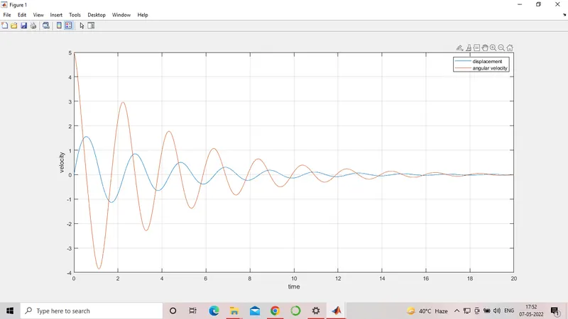
The Displacement (blue color) and Angular velocity (red color) is decreasing by the increased time,this is due to the introduction of Damper ie. Damping coefticient which absorbs the vibrations to make the body in equillibrium position.

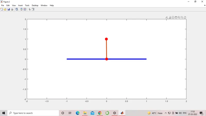
B. POSITION OF THE SETUP

Conclusion

1. The graph of Displacement and Angular velocity is plotted in Velocity v/s Time diagram.

2. Animation of Simple pendulum is created.

NOTE:-ANIMATION VIDEO WAS NOT UPLOADED BECAUSE I DONT KNOW HOW TO UPLOAD AVI FILE ON YOUTUBE