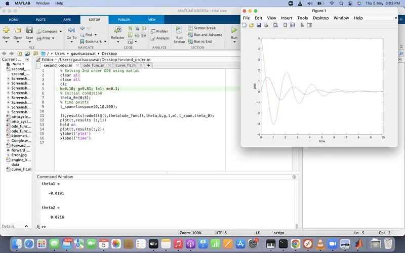
Week 3 - Solving second order ODEs
% second order differential equation can be described as diffrential
% equation which containss one or more functions of a n independent
% variable with derivatives of the function. 2nd order differential
% equation for a pendulum must be a function of ossicilation angle (theta )
% and length of pendulum,mass of pendulum with contionus damping
% coefficient which we have to take as input for function during coding.
% (d^2 theta / dt^2) + (b/m * dtheta/dt)+(g/l sin theta)= 0 {2nd order
% differential equation} where b= damping coeff.,m=mass,l= length of
% pendulum, g= gravity.

% Function code for calculating differential equation
function [dtheta_dt]= ode_func(t,theta,b,g,l,m)
theta1=theta(1)
theta2=theta(2)
dtheta1_dt=theta2;
dtheta2_dt=-(b/m)*theta2-(g/l)*sin(theta1);
dtheta_dt=[dtheta1_dt; dtheta2_dt];
end

% theta is taken as complied for representing theta 1 & theta 2
% Solution vector can be simplifed as
% d/dt[theta1 theta 2]= [ theta 2 -b/mtheta2-g/lsintheta1]

% Solving 2nd order ODE using matlab

clear all
close all
clc
b=0.10; g=9.81; l=1; m=0.1;
% initial condition
theta_0=[0;5];
% time points
t_span=linspace(0,20,700);
% for solving the ODE , ode45 function was used which is a predefined
% function in matlab for solving differential equations.ode45 takes 3
% inputs and t & theta shows that result of ode45 is based on time and
% angle.
[t,results]=ode45(@(t,theta)ode_func(t,theta,b,g,l,m),t_span,theta_0);
figure (1)
hold on
plot(t,results (:,1))
plot(t,results(:,2))
ylabel('plot')
xlabel('time')
legend('Angular displacement','Angular velocity')
% A loop gives a repetative control over a function and for loop is used to
% make conditions for the function to repeat where for loops requires
% initials like starting points of segment with end pints too. for starting
% a for loop we give first counter =1 as ct=1 and the for repetation we
% give next counter or incremental valve as ct=ct +1.

ct=1;
for i= 1:length(results(:,1))
    x0=0; y0=0;
    x1=l*sin(results(i,1));
    y1=-l*cos(results(i,1));
% plot curve for pendulam
    figure (2)
    plot([-1 1],[0 0],'linewidth',5)
    hold on
    plot([x0 x1],[y0 y1],'linewidth',3)
    hold on
    plot(x1, y1,'o','markersize',20,'markerfacecolor','y')
    title('Pendulam ossilations animation')
    axis([-1.5 1.5 -1.5 1])
    pause(0.02)
    hold off
M(ct)=getframe(gcf);
ct=ct+1;
end
% saving the animation in video format
% the final process is to capture the animation in video format or avi
% format f=and videowriter command is used for making it but video has to
% capture frames and must have cyclic pause so for capturing frames M is
% used and pause of 0.02 second is used.
movie(M)
videofile=VideoWriter('Pendulum_animation.avi','Uncompressed AVI');
open(videofile)
writeVideo(videofile,M)
close(videofile)
Link for the video : https://youtu.be/uxOI9tkeIwY