Week 3 - Solving second order ODEs

AIM :- to solve second order differential equation representing movement of pendulum with respect to time with damping using matlab.

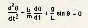
GOVERNING EQUATIONS:-

NOTATIONS :-

theta- angle of displacement

t- time

b- damping coefficient

g- acceleration due to gravity

l- length of rope

m - mass of pendulum

SOLUTION:-

clear all
close all
clc

b=0.05;%damping coefficient
g= 9.81; % acceleration due to gravity
l=1; %length of arm
m=0.1; %mass of object

%initial condition
theta_0= [0;3];

%time points
t_span= linspace(0,20,500);


%solving ode
[t,results]= ode45(@(t,theta)ode_func(t,theta,b,g,l,m),t_span,theta_0);

plot(t,results(:,1))
hold on
plot(t,results(:,2))
ylabel('plot')
xlabel('time')

EXPLAINATION :-

in first four lines we gave input of values of mass , acceleration due to gravity,damping coefficient and mass of object

then we gave input of displacement and velocity at theta = 0, (;) indicates that it is an column vector with values of displacement and velocity 0 and 3 respectively.

then we have to enter thr values of time for which we have to calculate theta so we used (t_span) to indicate time span and used linspace command to give it a span of 0 to 20 seconds with 500 intervals.

now, for solving derivative

ode45@(t,theta) indicate that this derivative is an function of t and theta,

code_func(t,theta,b,g,l,m) is a pre defined function

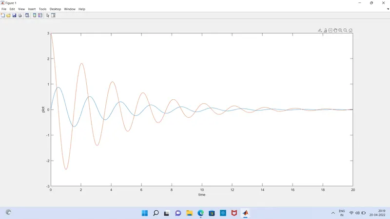
then we used plot command time with velocity and displacement outputs respectvely, which yielded following results.

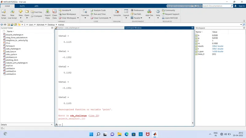
syntactical errors occured during coding is this