Solving second order ODEs

AIM:

To simulate the transient behavior of a simple pendulum and create an animation of its motion.
Below is the figure of the simple pendulum :

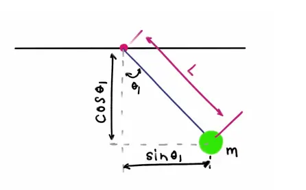
Below is the second-order differential equation for a simple pendulum:

Input Values:

b=0.05 (Damping coefficient)
g=9.81 (gravity in m/s^2)
l=1 (Length of pendulum in meter)
m=1 (Mass in Kg)

In initial condition Let's take,

Assume,

theta_0=[0;4]

Angular Displacement is 0

Angular Velocity is 4

t_span=linspace(0,20,300);

Time span is 0 to 20 sec, with 300 intervals.

Now solve ODE,

In matlab ode45 is the inubuilt solver for ODE,
Here ODE is the function of t and theta

t and theta are dependent and independent variables.

Below is the syntax for ODE,

[t,result]=ode45(@(t,theta) ode_function(b,g,l,m,t,theta),t_span,theta_0)
We have called function of name ode_function into it and give a name to ode_function as [dtheta_dt]

First Simplify,
Assume,

theta=theta1................(1)

So, dtheta_dt=dtheta1_dt

dtheta1_dt=theta2.................. (2)

Then, d^2theta_dt^2=d^2theta1_dt^2

=d_dt(theta2)

d^2theta_dt^2=dtheta2_dt...........(3)

So,

dtheta2_dt+(b/m)*theta2+(g/l)*sin(theta1)=0....(4)

dtheta1_dt=theta2........(5)

dtheta2_dt=-(b/m)*theta2-(g/l)*sin(theta1).......(6)

Now we have two equations,lets club into matrix form.

d_dt[theta1; theta2]=[theta2; -(b/m)*theta2-(g/L)*sin(theta1)]

and

dtheta_dt=[dtheta1_dt; dtheta2_dt]

To find the dtheta_dt matrix, we will create the ODE function
Note: theta is the solution array

function [dtheta_dt]=ode_function(b,g,l,m,t,theta)
theta1=theta(1);
theta2=theta(2);
dtheta1_dt=theta2;
dtheta2_dt=-(b/m)*theta2-(g/l)*sin(theta1);
dtheta_dt=[dtheta1_dt;dtheta2_dt]
end

Above this function, we have to find values for the result. The result has two columns, 1st for displacement and 2nd velocity.
That's why i am assigning,

theta1=theta(1) and theta2=theta(2)

The result part we will cover next,
Now, we will find values for displacement and velocity w.r.t. time in a matrix form of the table result.
Then call the above ode_function into the main program

close all
clear all
clc
b=0.05;
l=1;
m=1;
g=9.81;
theta_0=[0;4];
t_span=linspace(0,20,300);
[t,result]=ode45(@(t,theta) ode_function(b,g,l,m,t,theta),t_span,theta_0);

% @(t,theta)__defines it as a function as t, nad theta
% ode_function__defines the function which we defined in another program
figure(1)
hold on
plot(t,result(:,1),'color','r');% plotting the 1st coloumn results
plot(t,result(:,2),'color','b');% plotting the 2nd coloumn results
xlabel('Time')
ylabel('Displacemt/Velocity')
legend('Displacement','Velocity')
grid on

Results:

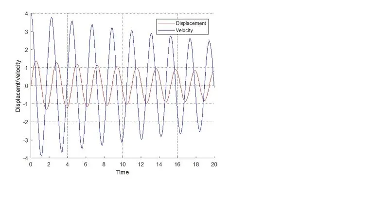
Movie Creation

close all
clear all
clc
b=0.05;
l=1;
m=1;
g=9.81;
theta_0=[0;4];
t_span=linspace(0,20,300);
[t,result]=ode45(@(t,theta) ode_function(b,g,l,m,t,theta),t_span,theta_0);
figure(1)
hold on
plot(t,result(:,1),'color','r');
plot(t,result(:,2),'color','b');
xlabel('Time')
ylabel('Displacemt/Velocity')
legend('Displacement','Velocity')
grid on

% Animation code%
ct=1;
for i=1:length(t)


 x0=0;
 y0=0;

 x1=l*sin(result(i,1));
 y1=-l*cos(result(i,1));
 
 figure(2)
 plot([-2 2],[0 0],'linewidth',3,'color','r');
 line([x0 x1],[y0 y1],'linewidth',4);

 axis([-2 2 -2 2])

 hold on
 plot(x1,y1,'o','markers',20,'markerfacecolor','g');
 hold off

 grid on
 pause(0.03);


 M(ct)=getframe(gcf);

 ct=ct+1;
end
movie(M)
videofile=VideoWriter('Second_order_ODE.avi','uncompressed avi')
open(videofile)
writeVideo(videofile,M)
close(videofile)

Conclusion:

Solving the second-order ODE is carried out