Week 3 - Solving second order ODEs

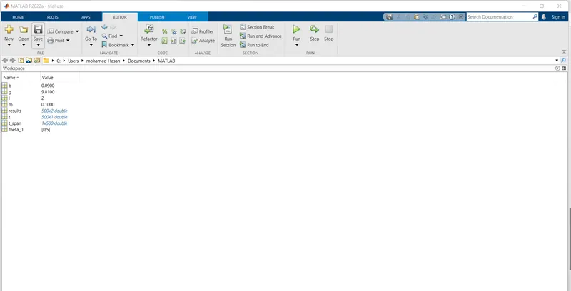
close all
clear all 
clc

b=0.09;
g=9.81;
l=2;
m=0.1;
% initial condition 
theta_0 =[0;5];

% time points
t_span= linspace(0,10,500);

 % solve ODE
 [t,results] =ode45(@(t,theta)ode_func(t,theta,b,g,l,m),t_span,theta_0);


 plot(t,results(:,1))
 hold on
 plot(t,results(:,2))
 xlabel('time')
 ylabel('plot')

EXPLANATION OF THE CODE ;
			*Before start thr program using clear all,close all,clc commanf.
			*Next step is to define the inputs and variabeles.
			*The damping coefficient,gravity,length of the spring nad mass of the bob have all been defined.
			*Next step is to solve the ODE ,it is a function in matlab that solves ordinary or partial differential equation using a numerical method.
			*The function takes three inputs .The inputs are the function to be integrated,the time span and the initial condition .
			*[t,results]means that the results that have been calculated with rspect to time.
			*After calculating the results ,a grafh has to be plotted.The grapg contains two plots .one is displacement with respect to time and anothe one
velocity with respect to time.