Week 3 - Solving second order ODEs

Attached Video----

https://drive.google.com/file/d/1sbAAV8qO1rTkdsR8sWktuSt6TiZmmLIN/view?usp=sharing

% A program to simulate the pendulum motion
% ODE that represent the equation of motion of simple pendulum is considered

%Initializing with to clear all the memory, close all files, figures and
%clear the common window screen.
clear all
close all
clc

%In the above equation,g = gravity in m/s2, L = length of the pendulum in m,
% m = mass of the ball in kg,b=damping coefficient.
%intial condition
b=0.05;
g=9.81;
l=1;
m=0.1;

%Intial condition--angular displacement=0 m, angular velocity =3 rad/sec at t=0
theta_0=[0;3];

%time points
t_span=linspace(0,20,500);
% start at 0 end at 20 seconds with 500 divisions
% Solving Oridinary Differential equation using ODE and calling the
% function that represents the the velocity and accelearion in matrix which
% when solved gives angle displacement and velocity repectively
[t, results]=ode45(@(t,theta) ode_func(t, theta,b,g,l,m),t_span,theta_0);
% In the answer t is the time divsion and results has two coloumn first has
% values for displacement angle and second for angular velocity.
% Defining an array A which will store all angular displacement
A=results(:,1);
% Intializing the counter within for loop
ct=1;
for i=1:length(A)
THETA1=A(i);
% Start point of the pendulum that is basically fixed
x0=0;
y0=0;
% X1 Y1 X2 Y2 coordinate in graph values
% Cos is used in y with negative and sin in x, since we want the
% position of pendulum around negative y axis
y1=-(l*cos(THETA1));
x1=(l*sin(THETA1));
% All these points are used to show fixed support and
% make the simulation more attracting and realistic
x2=-1.5;
x3=1.5;
y2=0;
y3=0;
x4=-1.5;
x5=1.5;
y4=0.03;
y5=0.03;
x6=-1;
x7=-1;
x8=1;
x9=1;
y6=0;
y7=3;
y8=0;
y9=3;

%figure(ct) to have differen plots
% Various points are added in this
% Linewidth to have increased size of lines
% Markindices with circular marker at every second point of line,
% though i have used in a way to hide for others line from screen
% MarkerSize, MarkerFaceColor ,MarkerEdgeColor to add characteristics
% to graph
plot([x0 x1],[y0 y1],[x2 x3],[y2 y3],[x4 x5],[y4 y5],[x6 x7],[y6 y7],[x8 x9],[y8 y9],'linewidth',3,'MarkerIndices',2,Marker='o',MarkerSize=15,MarkerFaceColor='m',MarkerEdgeColor='k',Color='k' )
% Axis to hide unnecsaary thing and show clear picture
axis([-1 1 -1.5 0.1]);
% Because we dont want values of axis it doesn't llook good
axis off

pause(0.01) %to see slow plotting
% M array to store the frames of graph shown in figure each time.
% gcf is used to capture interior of fiure window, excluding menu and
% toolbar
M(ct)=getframe(gcf);
% Increasing the position in array using counter ct to store second,
% third upto n frames till the for loop is designed for.
ct=ct+1;
end

movie(M)
%Naming the videofile and creating it in particular format
videofile=VideoWriter('Ode_pendulum','Uncompressed AVI');
% Openig the file called using temporary variable
open(videofile)
% Writing to the file using M array
writeVideo(videofile,M)
% Finally closing the same.
close(videofile)

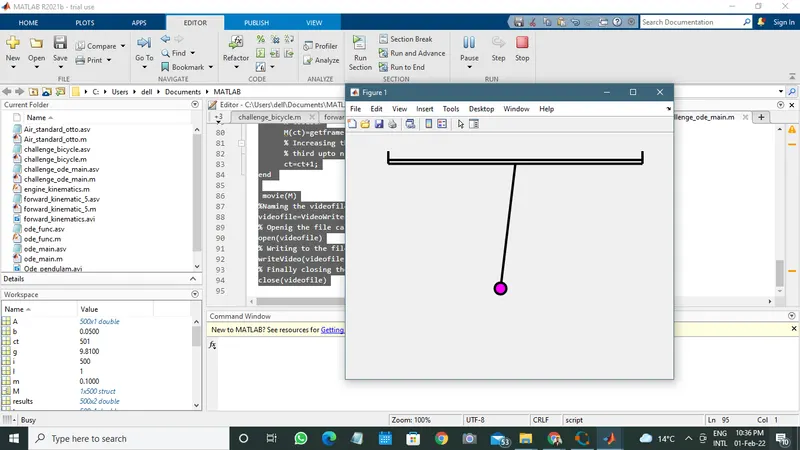
I wanted to make it more realistic as shown in the animation. So, I used various things. I was trying to show the fixed support as well. I have tried to show best according to my knowledge. But i think there will be some better also. Because this doesn't look good. Problem is that if i use hold on command then all the plots are hold. So, I had this solution in my mind.