Week 3 - Solving second order ODEs

Aim: Write matlab code to animate the motion of simple pendulum

Theory : In Engineering, ODE is used to describe the transient behavior of a system. A simple example is a pendulum.The way the pendulum moves depends on the Newtons second law. When this law is written down, we get a second order Ordinary Differential Equation that describes the position of the "ball" w.r.t time.

Governing equation :

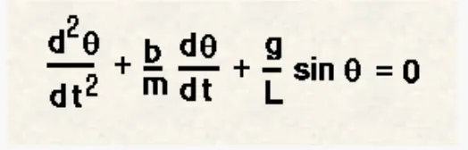
In the above equation,

g = gravity in m/s2,

L = length of the pendulum in m,

m = mass of the ball in kg,

b=damping coefficient.

L=1 metre,

m=1 kg,

b=0.05.

g=9.81 m/s2.

Objective: Simulate the motion between 0-20 sec, for angular displacement=0,angular velocity=3 rad/sec at time t=0.

at t = 0, displacement = 0 , angular velocity = 3 rad/sec

Main code:

clear all
close all
clc
g = 9.81;
L = 1;
b = 0.05;
m = 1;
ode_fun = @(t,theta)[theta(2);...
                     -((g/L)*sin(theta(1)))-((b/m)*theta(2))];
tspan = linspace(0,20,500)
theta_0 = [0,3];

[t,Theta] = ode45(ode_fun,tspan,theta_0);
figure(1)
subplot(2,1,1)
plot(t,Theta(:,1),'color','r','linewidth',3)
xlabel('time(s)')
ylabel('displacement(rad)')
subplot(2,1,2)
plot(t,Theta(:,2),'linewidth',3)
xlabel('time(sec)')
ylabel('angular velocity(rad/sec)')



x0 = 0 
y0 = 0


ct = 1;
for i = 1:length(tspan)
    x1 = L*sin(Theta(i,1));
    y1 = -L*cos(Theta(i,1));
figure(2)
    plot([x0 x1],[y0 y1],'linewidth',4,'color','r')
    hold on
    plot(x0,y0,'Marker','o','MarkerSize',3,'MarkerFaceColor','y')
    plot(x1,y1,'Marker','O','MarkerSize',20,'MarkerFaceColor','g')
    plot([-1 1],[0 0],'linewidth',6,'color','b')
    hold off
   axis([-3 3 -2 2])
   legend('arm','fixed point','bob','support rod')
   grid on
    pause(0.1)
    M(ct)=getframe(gcf);
    ct = ct+1;
    
end

movie(M)
videofile = VideoWriter('simple_pendulum.avi','Uncompressed AVI')
open(videofile)
writeVideo(videofile,M)
close(videofile)

Steps :

1. Convert the second order ode into first order ode and store the equations we get in an array.
2. Give inputs to different parameters
3. solve the equations using ode45
4. create ode_fun to store the equations we got by changing second order ode to first order ode
5. give tspan and initial values of displacement and angular velocity inside ode45
6. now the result we get is stored in columns of 2, first column corresponds to displacement and second column corresponds to angualr velocity.
7. plot Time vs dispalcement and Time vs angular velocity
8. give x0 and y0 values for fixed point, set counter (ct) as 1
9. use for loop from 1 to length of time
10. calculate values of x1 and y1 at each insatnce of time, plot them.
11. store each frame of plot inside array M
12. increase counter by 1
13. for loop ends when length of time is reached
14. create movie using matlab commands.

Results :

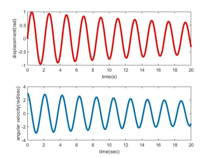
Animation : https://youtu.be/DRe99RZtFD8