Week 3 - Solving second order ODEs

Aim:

To determine the Simple Pendulum using 2nd Order Differential Equation .

Objective:

1.Writing Code to Solve the 2nd Order Differential Equation.

2.This Code representing to Simple Pendulum.

3.Create a Animation for Simple Pendulum Damping motion.

Simple Pendulum:

Simple Pendulum is a Weight suspended Pivot such that it can swing freely.

An Ideal simple pendulum is defind as the heavy point mass (bob) suspended inextensible string from a perfect rigid support and oscillating freeely without any friction.

Characteristics:

When the mass oscillating for long time the amplitude of Oscillation becomes smaller and gradually the oscillations becomes stop.

The decrease the amplitude is due to air resistance & friction the point suspension.These are called Damping Oscillation or Oscillationary motion.

The max.displacement of pendulum on either side from it's mean position in horigental direction is called Amplitude.

Period of Oscillation or Time period(T) and time taken to complete one Oscillation .

T = `2*pi*root()(l/g)`

l = Length

g = Gravity

Frequency of Oscillation is No. of Oscillations performed in one second and it's units are cps or Hertz

f = 1/T

A pendulum with a period of oscillation equal to 2 seconds is known as seconds pendulum.

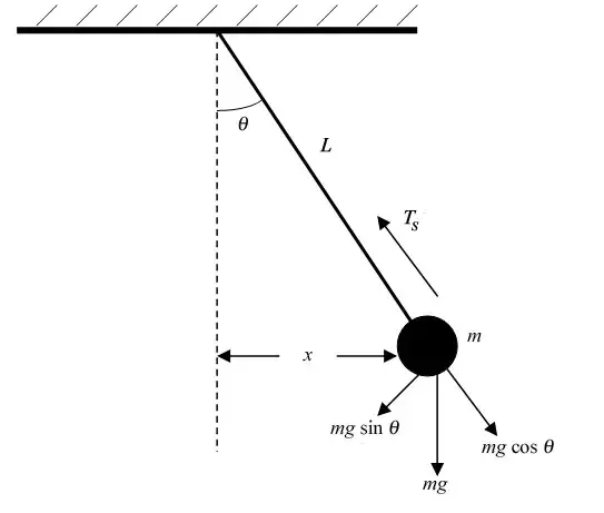
Fig.1. Simple Pendulum Motion

Pendulum mass is suspended from end of rod with Length L is swinging in vertical plane. Let `theta` be the angle measured in radian from vertical right side to be positive .

W = -mgsin`theta` acting on mass direction opposite to the motion.

Programme:

function [dtheta_dt] = ode_func(t,theta,b,g,l,m)


theta1 = theta(1);
theta2 = theta(2);
dtheta1_dt = theta2;
dtheta2_dt = -(b/m)*theta2 - (g/l)*sin(theta1);
dtheta_dt = [dtheta1_dt ; dtheta2_dt];

end 

The simplefied 2nd order ODE into 2 system of 1st Order ODE programme written above and it taken as a function.

% clearing and closing all Variables ,plots Command window 
     clear all
     close all 
     clc
     
 %Inputs 
 b = 0.05; % Damping Coefficient 
 g = 9.81;  % Gravity m/s^2
 l = 1;     % length m
 m = 0.1;   % mass in Kg
 
 % Initial condition
 theta_0 = [0,3];  % Intial Displcement , Intial Velocity
 
 %time points
 t_span = linspace(0,10,500);
 % solve ODE
 [t,results] = ode45(@(t,theta) ode_func(t,theta,b,g,l,m),t_span,theta_0);
 
 subplot(2,2,1)
 plot(t,results(:,1),'color','b')
 hold on
 plot(t,results(:,2),'color','r')
 hold off
xlabel('Time')
ylabel('Displacement')
subplot(2,2,2);
 plot(results(:,1),results(:,2));
 xlabel('Position-Radians')
 ylabel('Angular Velocity')
 ct = 1;

 for i = 1:length (results(:,1))
   x0 = 0;
   y0 = 0;
   x1 = l*sin(results(i,1))
   y1 = -l*cos(results(i,1))
    subplot(2,2,[3,4])
   plot([-1 1],[0 0],'linewidth',4,'color','k')
   hold on
   line([x0 x1],[y0 y1],'linewidth',2,'color','b')
  hold on
   plot(x1,y1,'-o','markers',20,'markerfacecolor','r')
   axis([-1.5 1.5 -1.5 0.5])
   pause (0.0003);
  grid on
    q(ct) = getframe(gcf);
    text = sprintf("pendulum%d.png",ct);
    saveas(1,text)
    hold off
    ct = ct+1
 end

 movie(q)
 videofile = VideoWriter('Pendulum_damped.avi','uncompressed avi')
 open(videofile)
 writeVideo(videofile,q)
 close(videofile)

Code Explanation:

1. Frist of all Clear and close all the plots,Variables,Command line window.

2.Given Inputs are

b = 0.05 Damping Coefficient
g = 9.81 Gravity m/s^2
l = 1 length m
m = 0.1 mass in Kg

3.Initial Condition for Displacement and Velocity given as Theta_0 = [0,3].

4.The time rate value is T_span = linspace (0,10,500) to create Multiple values .

5. Solving ODE used ODE 45 Inbulit solver of ODE . The main inputs are time and angle Solving Function ODE t,theta, and all intial conditions and inputs then time rate and theta_0

6.Subplot used to Create multiple plots in Single window.

7.Ploting the Results of 1st and 2nd Columns and with Labels.

8. To create an animation with all values used loop command .

9. Intial co ordinates are origin and Simple pendulum damping with X1,Y1 values.

10. For bob used marker command with red colour given grid on for plot.

11.Pause animation value mentioned.

12.getframe is used to get all recentframes are plotted.

13.And fianally Created movie file.

Animation Link:

https://youtu.be/n7vD_vmSyz4

Conclusion:

The Simple Pendulum Solved by using 2nd order ODE with with ODE inbuilt Sovler ODE 45 and The Dispalcement with respect to time .So that Velocity Showed above of Motion of Simple Pendulum starts with O and ends with 5 and Time in Seconds. And The Animation Created with Red Colour in the Fig. is mass Suspended from fixed rigid postion with inextensible rod. It 's Motion is animated according to the inputs.