Week 3 - Solving second order ODEs

Aim: To write a program that solves the following ODE. This ODE represents the equation of motion of a simple pendulum with damping

Where,

g = gravity in m/s2,

L = length of the pendulum in m,

m = mass of the ball in kg,

b=damping coefficient.

Simulate the motion between 0-20 sec, for angular displacement=0,angular velocity=3 rad/sec at time t=0. Use this information to animate the motion of the pendulum.

Theory: An Ordinary Differential Eqn is an eqn whohc consists of one r more functions of one independent variable along with their derivatives. It is divided into 3 types:

• Autonomous ODE
• Linear ODE
• Non-linear ODE

Code:

import numpy as np
from scipy.integrate import odeint
import matplotlib.pyplot as plt
import math

#function that returns dz/dt
def model(theta,t,b,g,l,m):

	theta1 = theta[0]
	theta2 = theta[1]
	dtheta1_dt = theta2
	dtheta2_dt = -(b/m)*theta2 - (g/l)*math.sin(theta1)
	dtheta_dt = [dtheta1_dt, dtheta2_dt]
	return dtheta_dt

#constants

#damping co-efficient
b = 0.05
#acceleration due to gravity
g = 9.81
#length of pendulum, m
L = 1
#mass of the ball, kg
m = 1

#initial condition
theta_0 = [0, 3]

#time points
t = np.linspace(0,20,150)

#solve ODE
theta = odeint(model,theta_0,t,args = (b,g,L,m))

#plot results
plt.plot(t,theta[:,0],'b-')
plt.plot(t,theta[:,1],'r--')
plt.ylabel('Plot')
plt.xlabel('Time')
plt.legend(loc='best')
plt.show()

a = theta[:,0]
b = theta[:,1]
ct = 1

for i in a:
	x0 = 0
	y0 = 0

	x1 = L*(math.sin(i))
	y1 = -L*(math.cos(i))

	filename = str(ct) + '.png'

	ct = ct + 1

	plt.figure()
	plt.plot([-0.5,0.5],[0,0])
	plt.plot([x0,x1],[y0,y1])
	plt.plot(x1,y1,marker='.',markersize=30)
	plt.xlim([-1.5,1.5])
	plt.ylim([-1.5,1.5])
	plt.savefig(filename)

Explanation:

• Import math, scipy.integrate (for odeint), numpy and matplotlib classes.
• Inputs taken:

  • L=1 metre

  • m=1 kg

  • b=0.05

  • g=9.81 `m/s2`.

• Created a new function that returns dz/dt with theta, time, damping cofficient, acceleration due to gravity, length of pendulum and mass of pendulum as constants.
• This function calculations the first and second derivatives of theta 1 and theta 2 and returns the result of the formula below:
• Time points are calculated from 0 to 20, divided into 150 intervals.
• The result of the formula above is stored in avriable called theta.
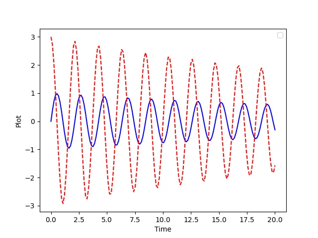
• Plot Results - Time on X axis, Displacement & Velocity on Y axis.
• We can observe the curve dampens quickly as the damping coefficient is increased above 0.05.
• In the next part of the program, to create animation, use a 'for' loop to get X and Y co-ordinates using trigonometric eqns as shown below:
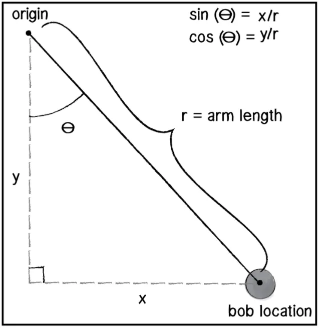
• (0.5,0.5) are hinge points. Plot the string of the pendulum, the bob (with markersize) and the top support.
• Using a counter variable ct, create and save a new plot with new name, with every iteration.
• Stich all the images to create an animation.

Results: The Displacement, Velocity vs Time Plot is shown below:

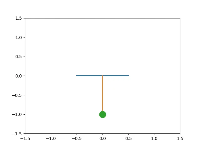
The simple pendulum motion is shown below: