Week 3: Flow over a backward facing step

• • Aim:-

  • To conduct a Computational Fluid Dynamics (CFD) simulation of Backward Facing Step (BFS) flow using CONVERGE CFD software, with post-processing carried out in ParaView.

  • To examine the influence of mesh grid resolution by simulating the BFS flow using three different mesh sizes.

  • To generate and compare velocity contours and pressure distribution for each mesh configuration.

  • To evaluate and analyze the performance of each mesh by plotting velocity profiles, pressure variations, mass flow rates, and total cell count.

  • To investigate the turbulent flow behavior in the BFS geometry and understand the flow separation and reattachment phenomena downstream of the step.

Introduction:

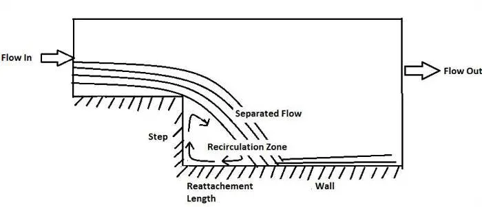
The backward-facing step (BFS) flow is a classic case in computational fluid dynamics that involves flow separation, reattachment, and recirculation due to sudden expansion in a channel. A fully developed flow enters the domain and encounters a sudden geometric step, leading to adverse pressure gradients, flow detachment, and the formation of a recirculation zone

BFS flows are commonly observed in many engineering applications, including airfoils, automotive aerodynamics, exhaust systems, diffusers, and heat exchangers. The flow behavior downstream of the step is influenced by step geometry, inlet conditions, turbulence levels, and thermal conditions.

The main features include:

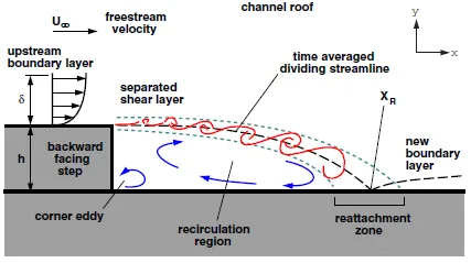
• Separation of the turbulent boundary layer.
• Formation of shear layers and vortices.
• Reattachment of the flow downstream.
• Pressure recovery after flow reattachment.

Geometry Creation:

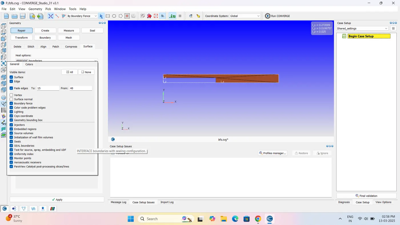
The BFS geometry was constructed in CONVERGE using the vertex-based modeling approach. The step geometry was created by:

1. Defining vertex coordinates.
2. Connecting vertices using triangle surfaces.
3. Extruding geometry in the Z-direction (depth = 0.02 m) using the "loft" function to generate a 3D domain.
4. Adjusting surface normals and validating geometry through diagnostics (checking for open edges, intersections, or isolated triangles).

Case Setup:

Simulation Settings:

• Solver Mode: Steady-State
• Simulation Mode: Full Hydrodynamic
• Physics Models Enabled: Momentum, Species Transport
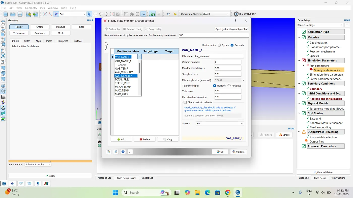
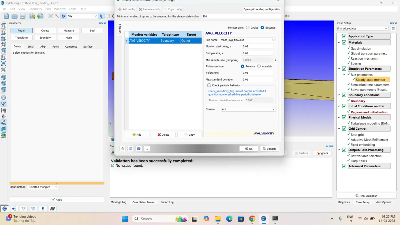
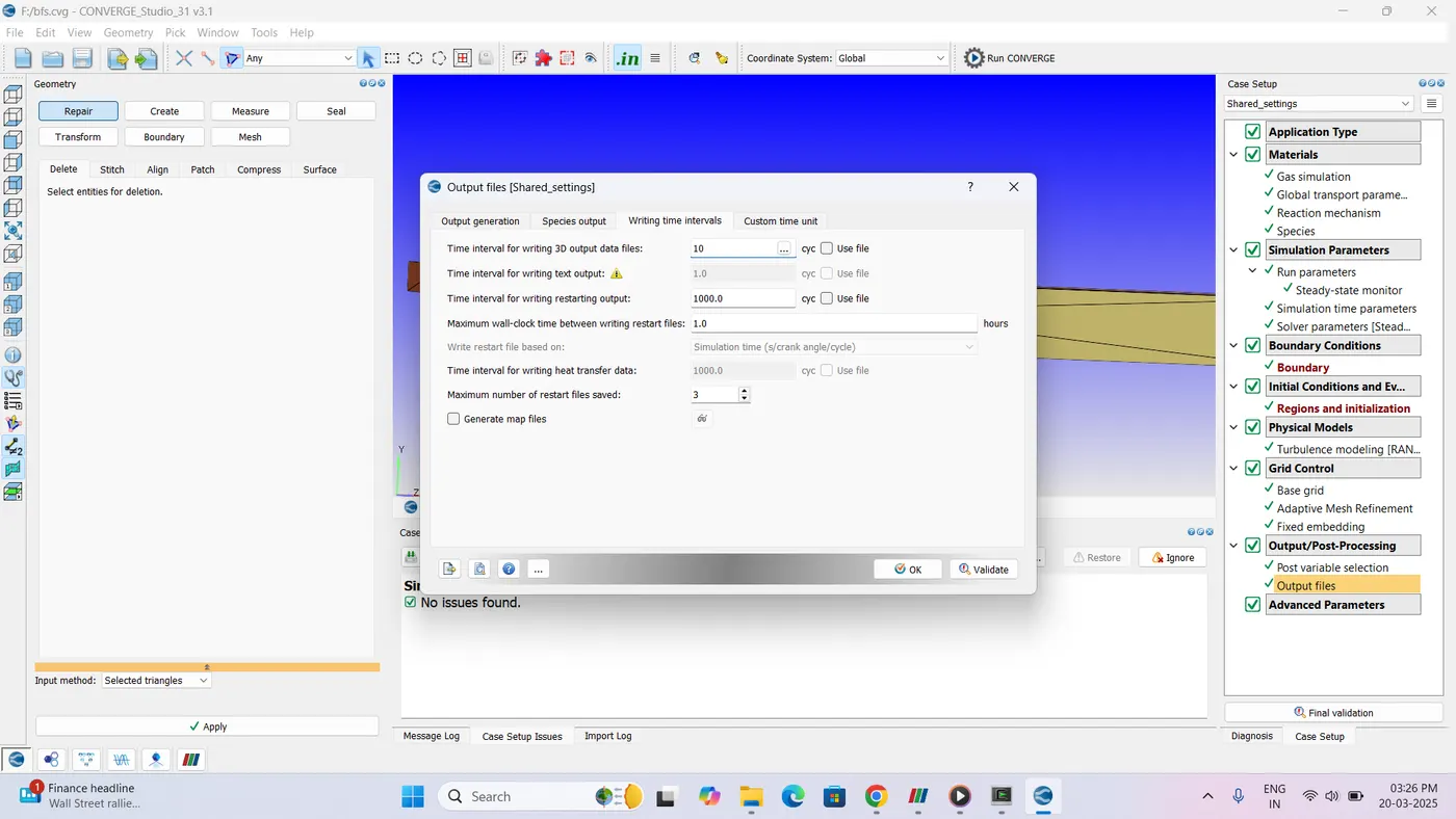
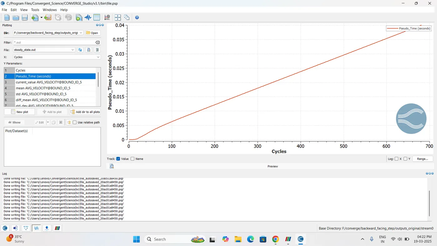
• Steady-State Criteria: 15,000 cycles
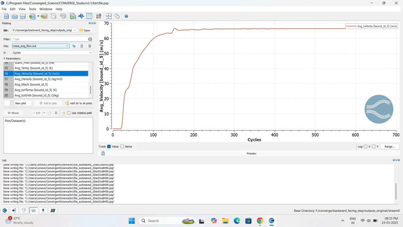
• Monitor Variables: Mass Flow Rate, Average Velocity

Time Settings:

• Start Time: 0 cycles
• End Time: 15,000 cycles
• Minimum and Initial Time Step: 1e-9 sec

Solver Parameters:

• Pressure-based Navier–Stokes Solver
• Default settings for other solver parameters

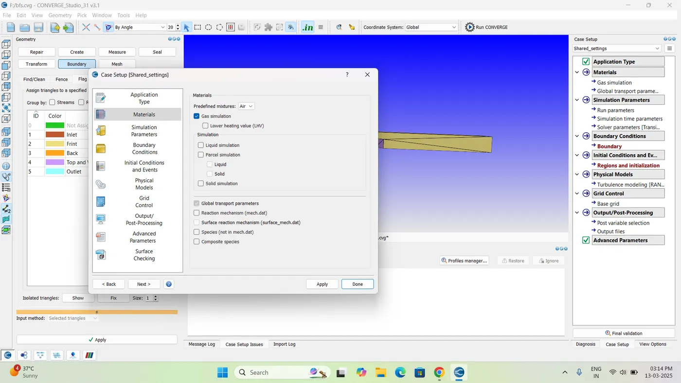
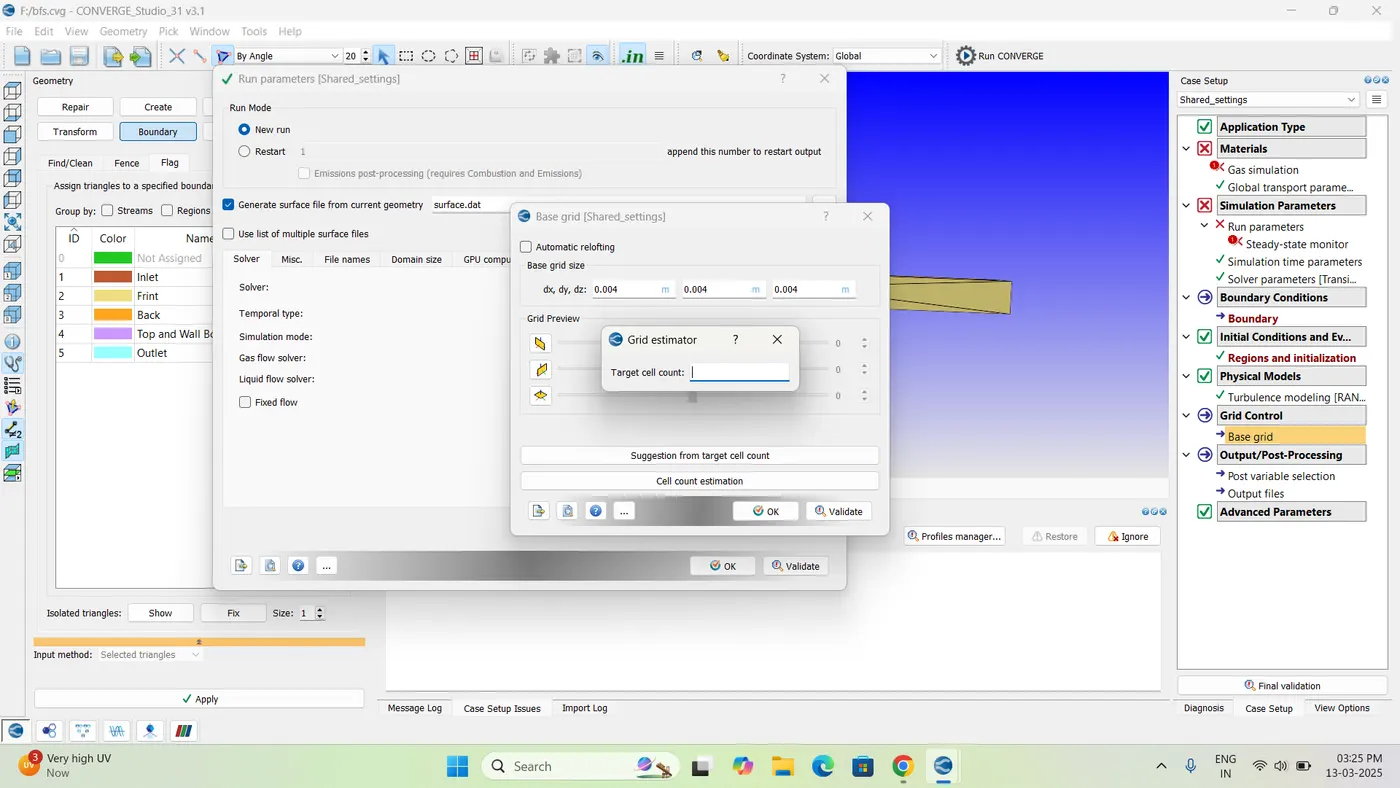
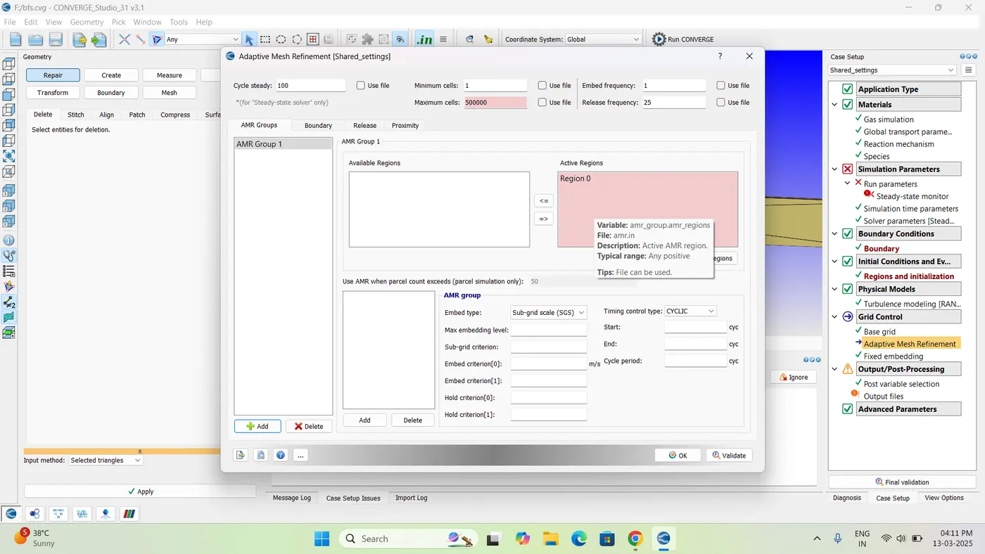
Initialization and Boundary Conditions:

• Initialization Region:

  • Temperature: 300 K
  • Pressure: 101325 Pa
  • Species: O₂ (23%), N₂ (77%)

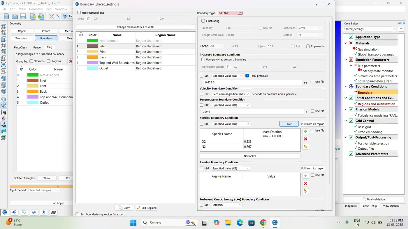
• Inlet Boundary:

  • Pressure: 110325 Pa
  • Temperature: 300 K
  • Type: Inflow

• Outlet Boundary:

  • Pressure: 101325 Pa
  • Temperature: 300 K
  • Type: Outflow

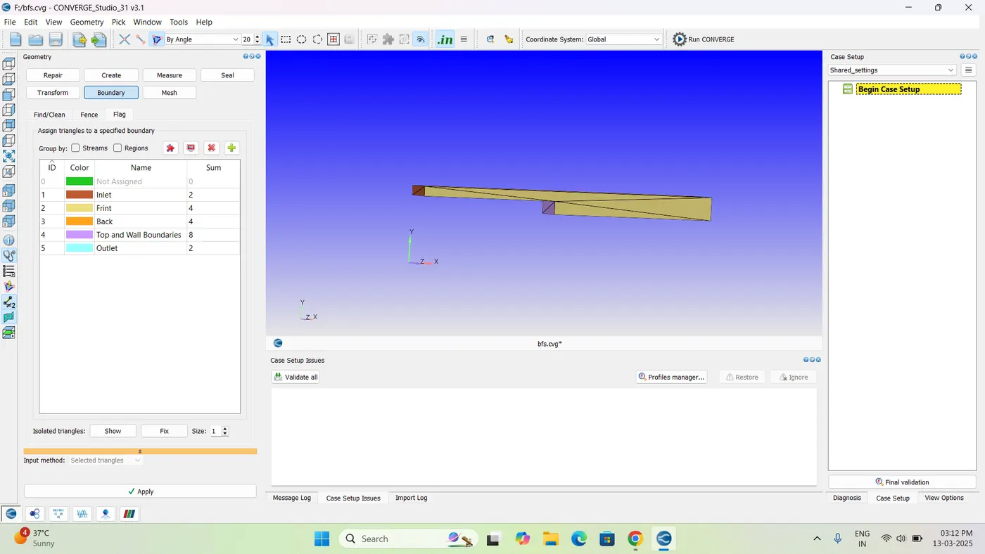
• Wall Boundaries:

  • Top & Bottom: Wall with law-of-the-wall condition, Temperature = 300 K
  • Front & Back: 2D Walls

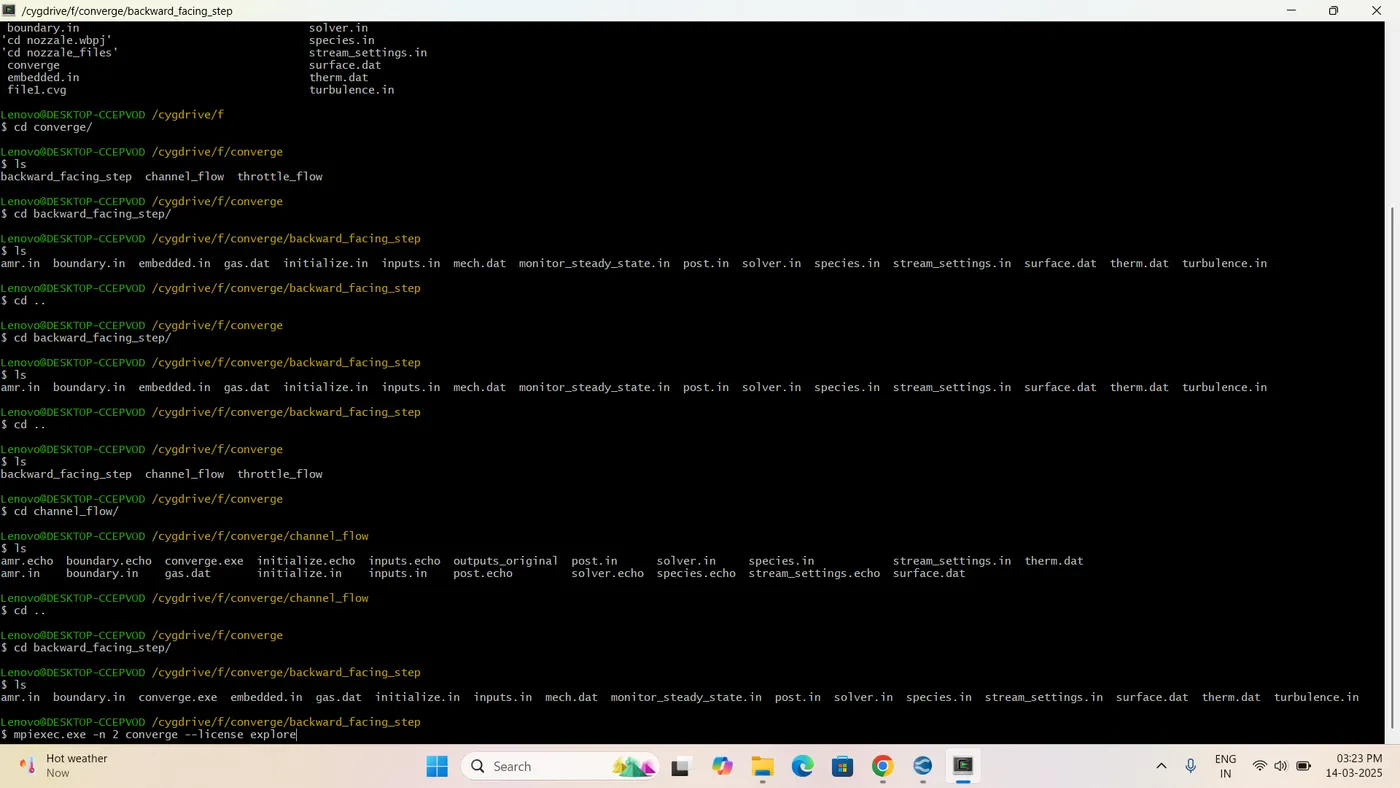
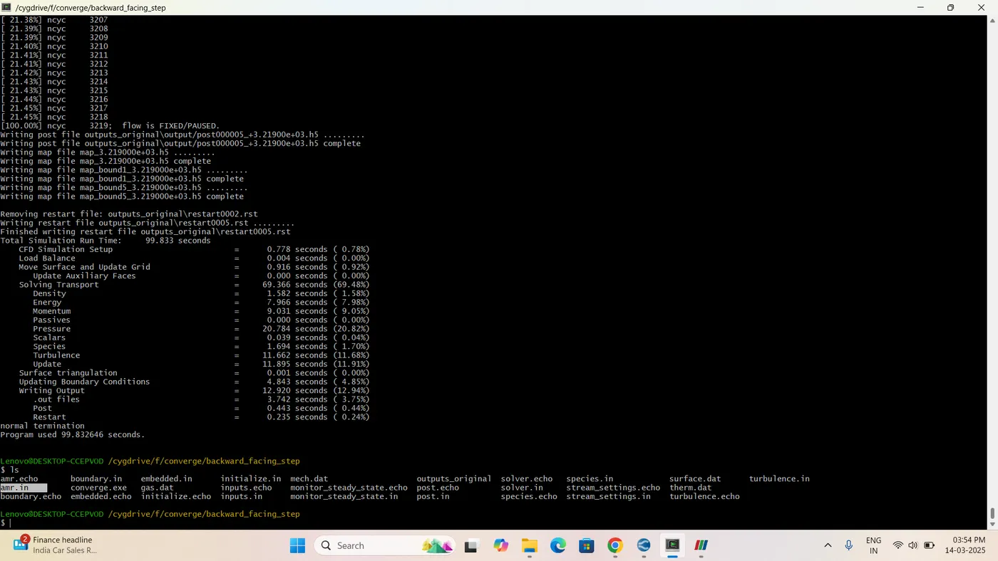
:- Reining program in cygwin

:- para view case setup

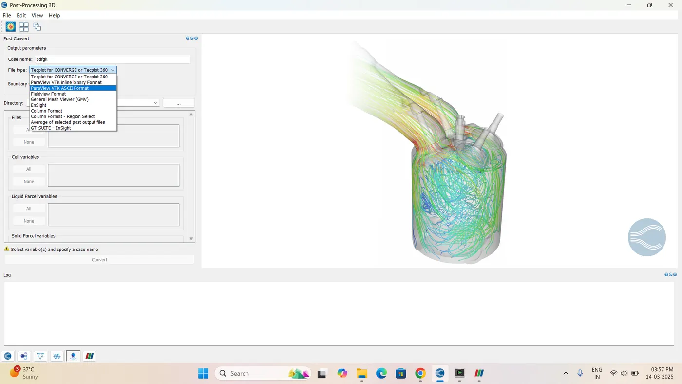
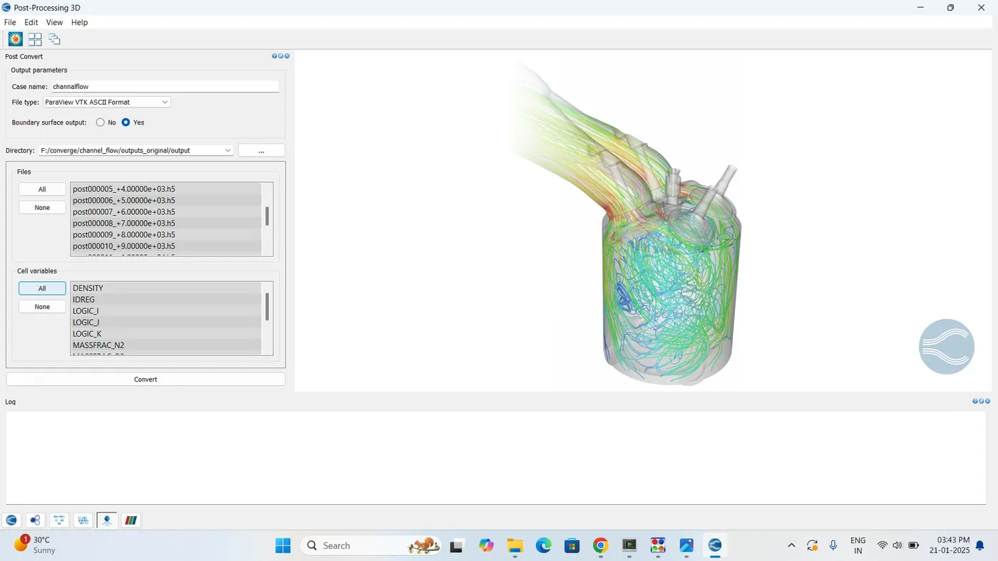
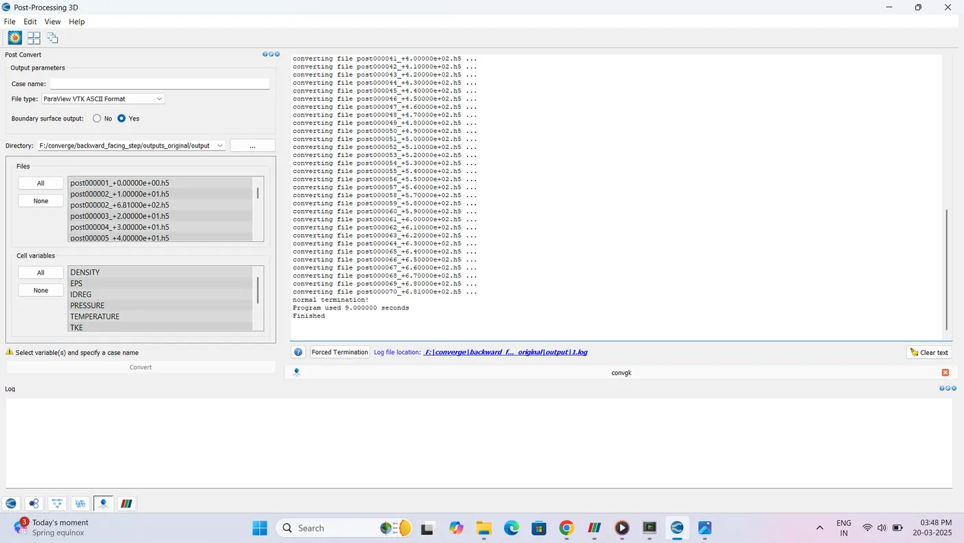
:- Opining paraview

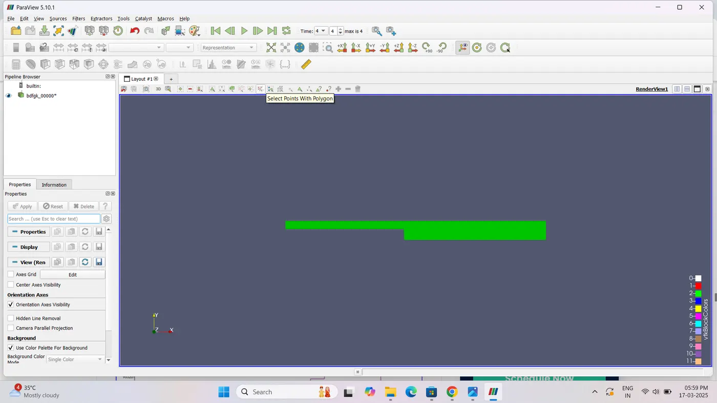
Grid Control:

Simulations were conducted for three uniform mesh sizes:

1. Case-I: dx = dy = dz = 2e-3 m
2. Case-II: dx = dy = dz = 1.2e-3 m
3. Case-III: dx = dy = dz = 1e-3 m

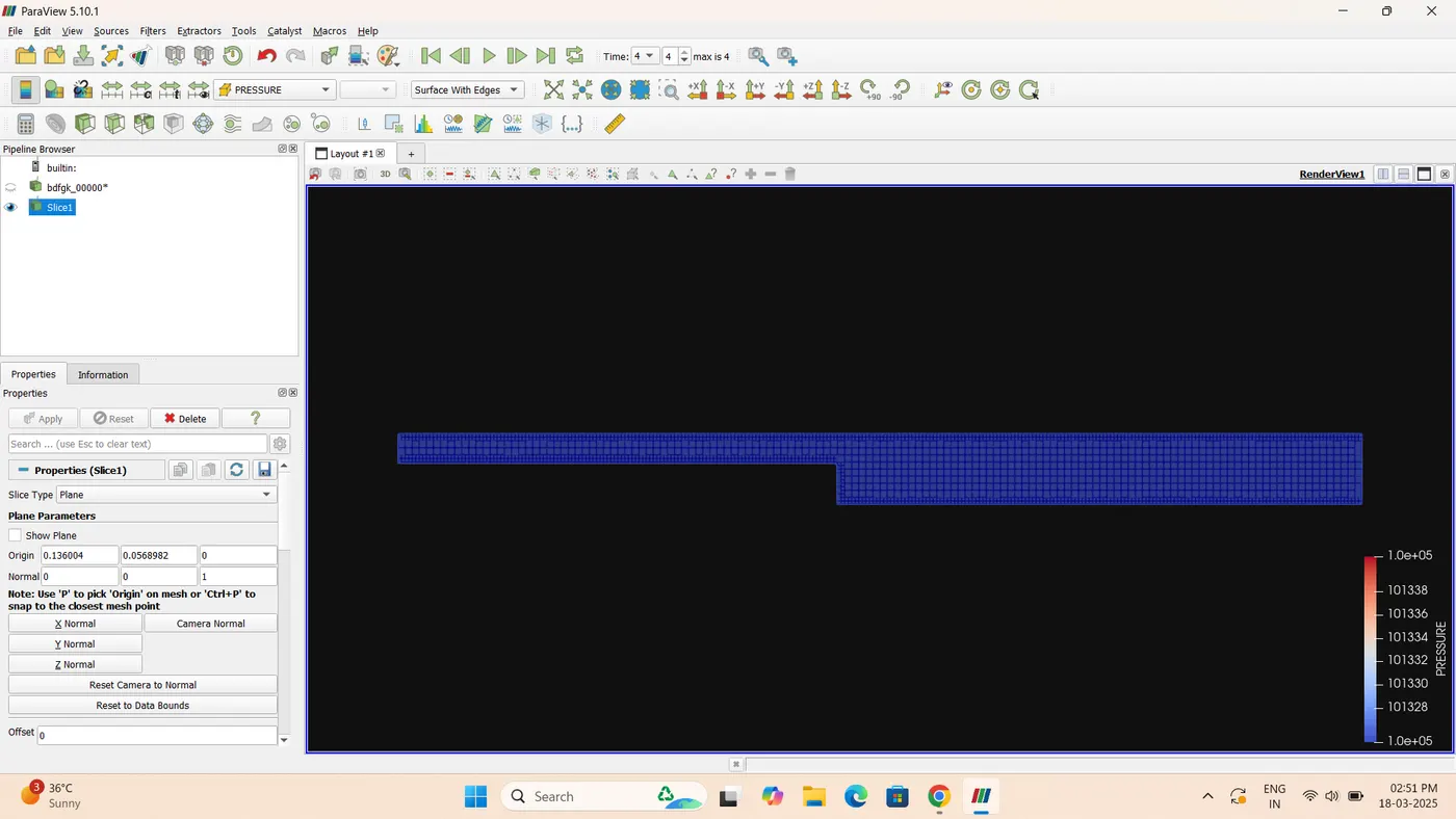
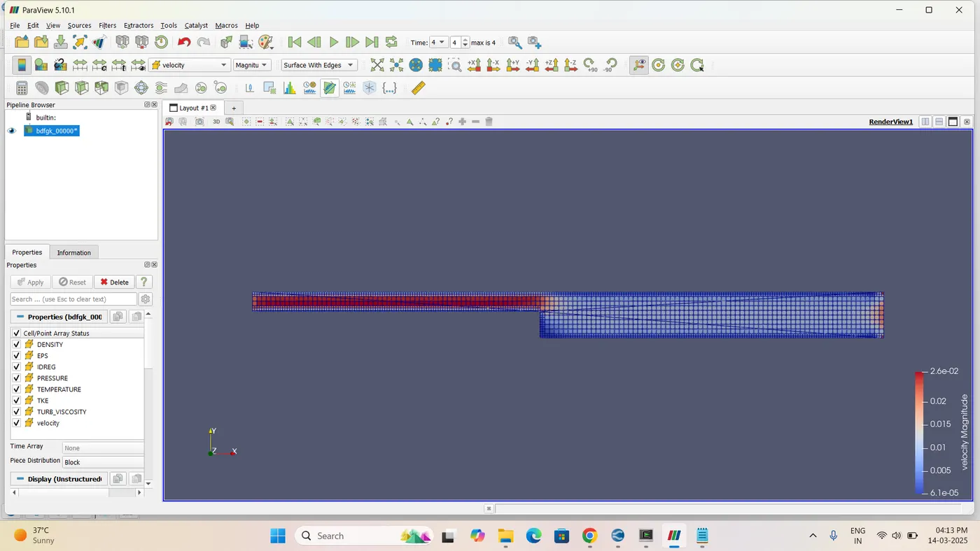
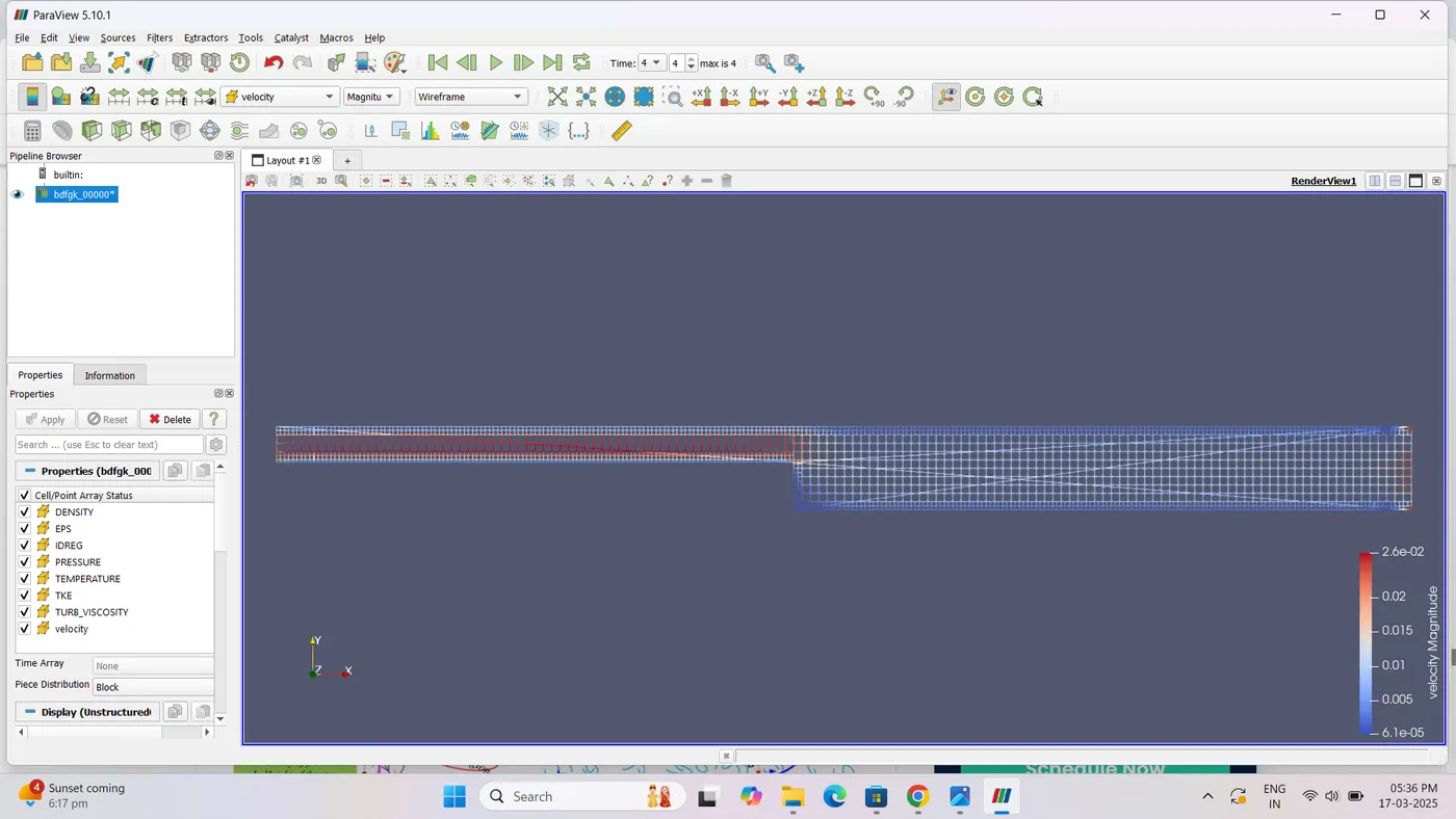
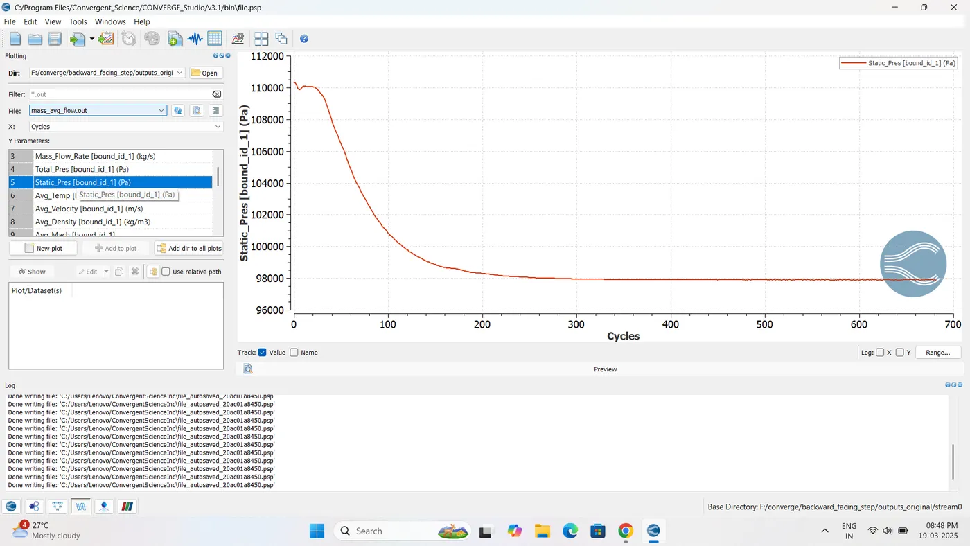
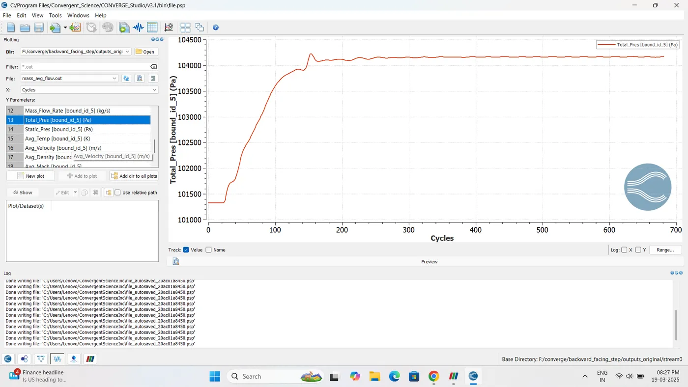
Pressure is high at the inlet and increases slightly near the step. After the step, it drops due to turbulence and flow separation caused by the adverse pressure gradient. The pressure gradually recovers and reaches a maximum at the outlet.

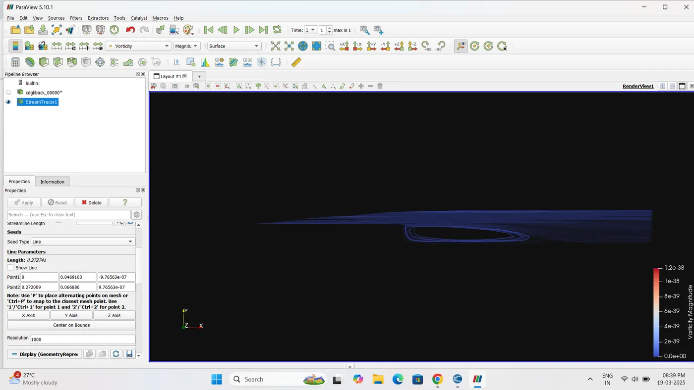
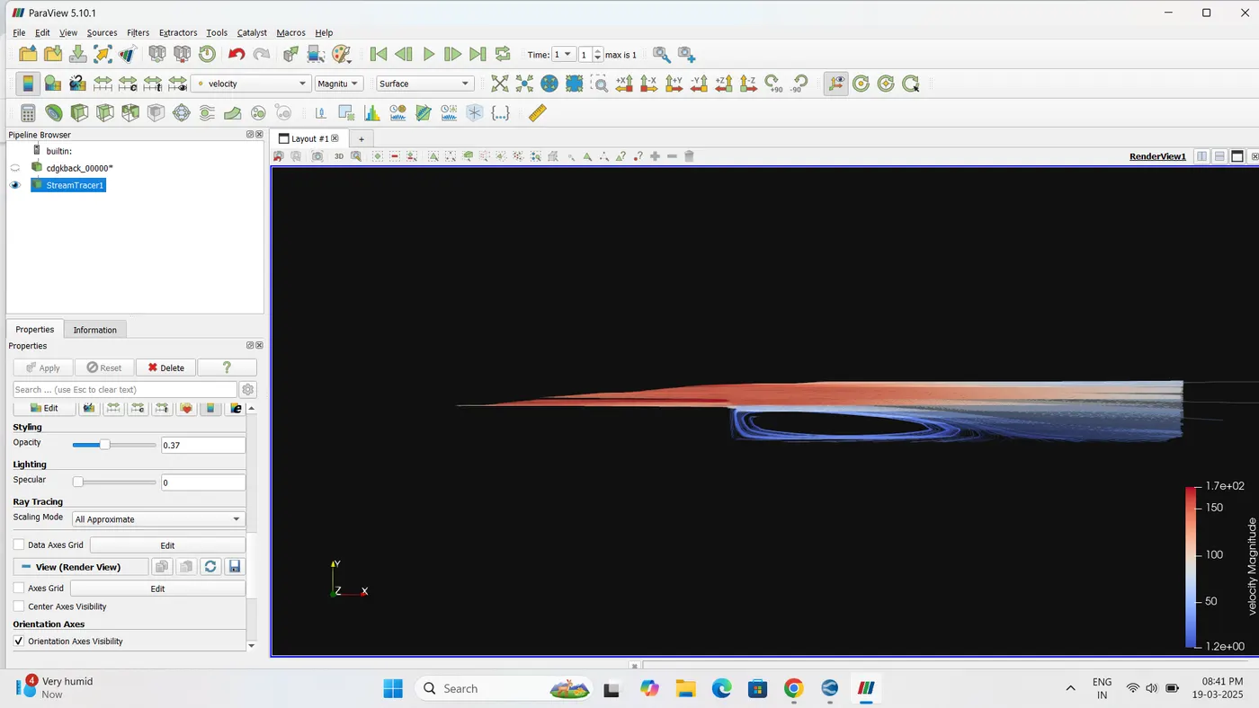
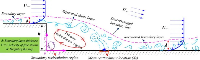
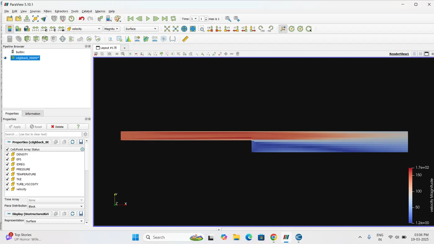
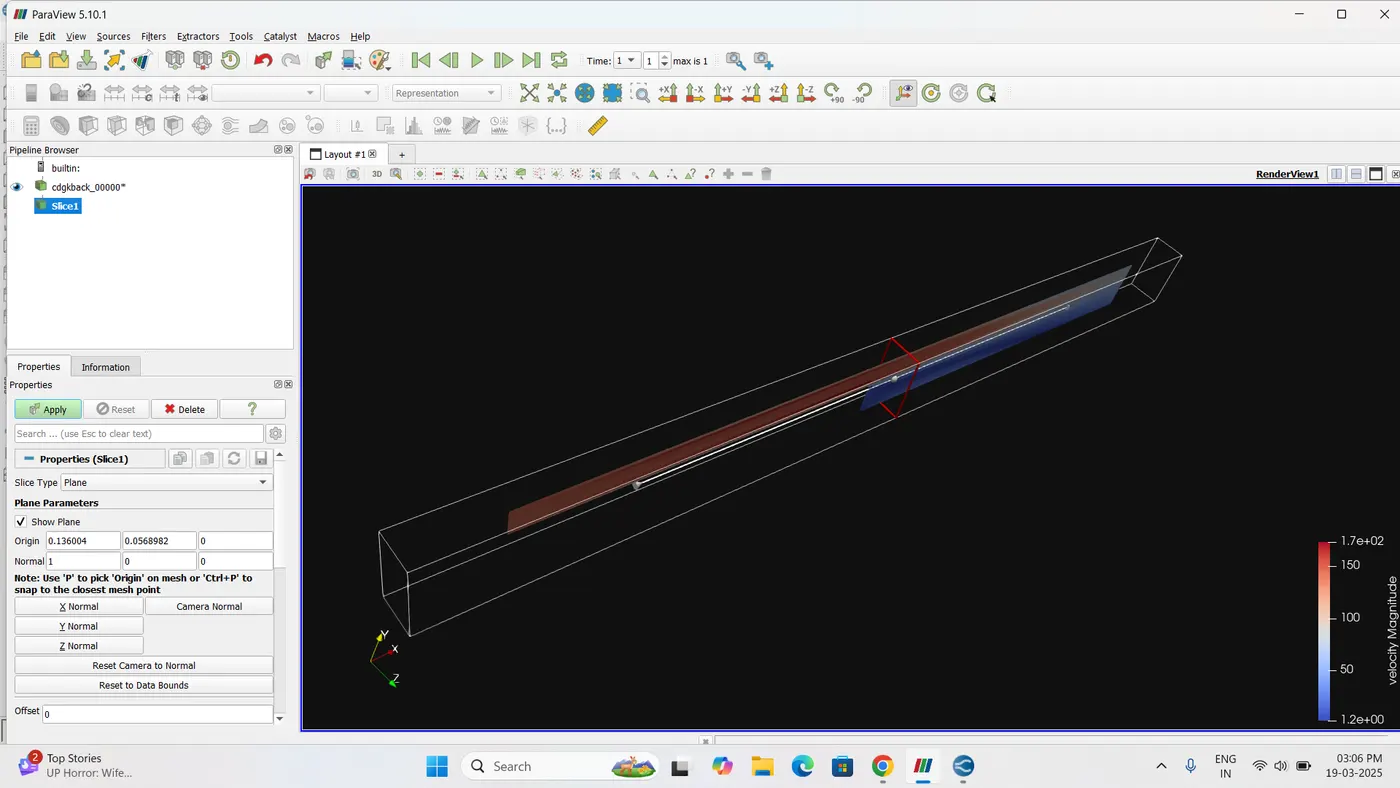
The velocity contour results clearly illustrate the typical flow behavior associated with backward-facing step geometry. Prior to the step, a boundary layer forms along the upstream wall. When the flow encounters the step, a sudden increase in cross-sectional area generates an adverse pressure gradient, leading to boundary layer separation and the formation of a shear layer.

This shear layer entrains low-velocity fluid from the near-wall region, resulting in a recirculation zone downstream of the step. A primary vortex is formed centrally within this zone, while a secondary vortex commonly develops at the step corner due to localized flow separation and shear interactions.

The adverse pressure gradient causes the shear layer to bend downward toward the wall. Some of the flow circulates in the recirculation bubble, while the rest continues downstream. The reattachment length, defined as the distance from the step to the reattachment point on the lower wall, characterizes the transition from separated to reattached flow. Beyond this point, the flow progressively stabilizes and exits the domain.

Plots for Different Mesh Sizes

For each of the three mesh grid sizes (Coarse, Medium, and Fine), the following plots should be presented and compared:

1. Velocity Profile Plot

• Plot velocity along a line (e.g., centerline or at a specific downstream location).

• Compare the velocity magnitude or velocity components (Ux, Uy) across the three mesh sizes.

• Helps in observing flow development, separation, and reattachment zones.

2. Pressure Distribution Plot

• Plot static pressure along the length of the domain (x-direction) for each mesh.

• Useful to study pressure drop and recirculation zones.

• Helps to identify any pressure losses or mesh-related discrepancies.

3. Mass Flow Rate Plot

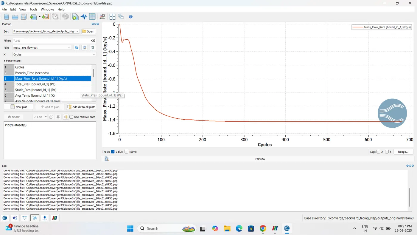
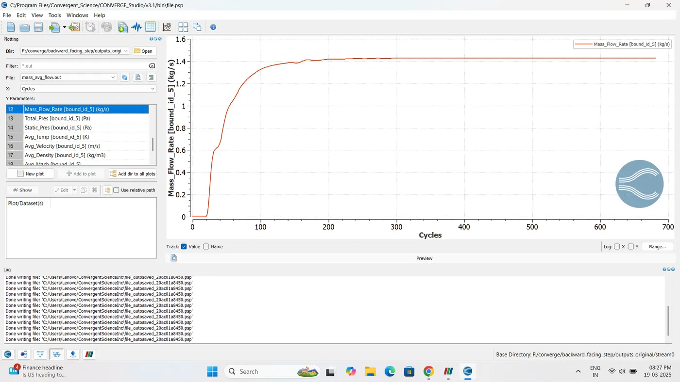
• Plot mass flow rate at the outlet for each mesh.

• Indicates how mesh size affects the conservation of mass and flow characteristics.

4. Total Cell Count Comparison

• A bar chart or table comparing the total number of computational cells in each mesh.

• Highlights the computational cost and resolution trade-off.

5. Contour Plots (Velocity & Pressure)

• Display contour plots of velocity magnitude and pressure for all three mesh sizes.

• Visual comparison helps understand how mesh refinement improves resolution of flow features like vortices, separation zones, and reattachment.

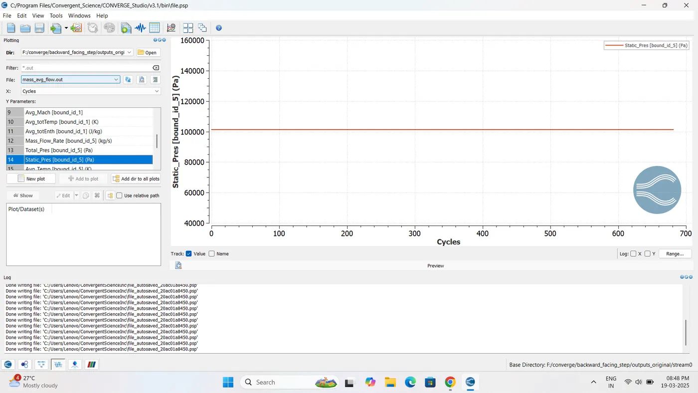
:-Stagnation Pressure Plot

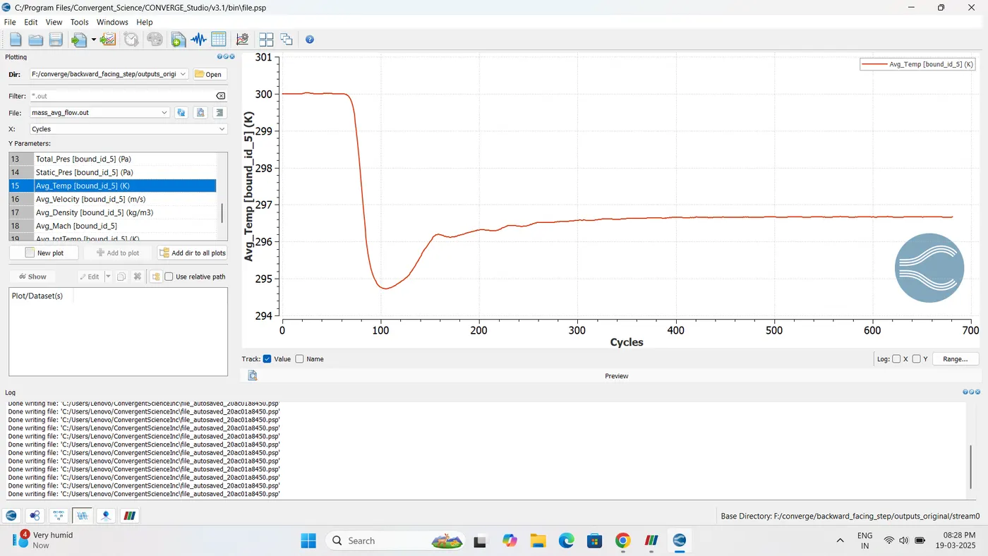
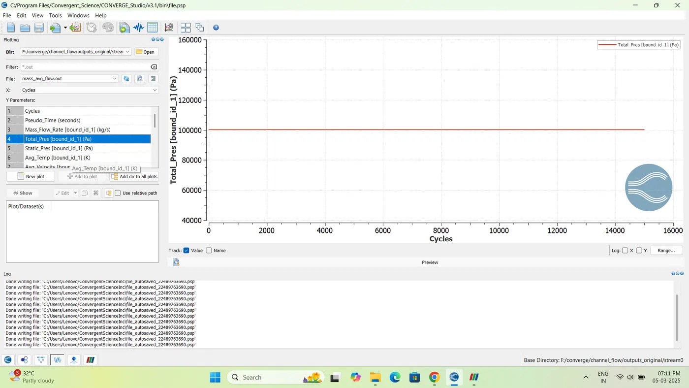
In the plot, we show how stagnation pressure changes along the length of the domain (from inlet to outlet).

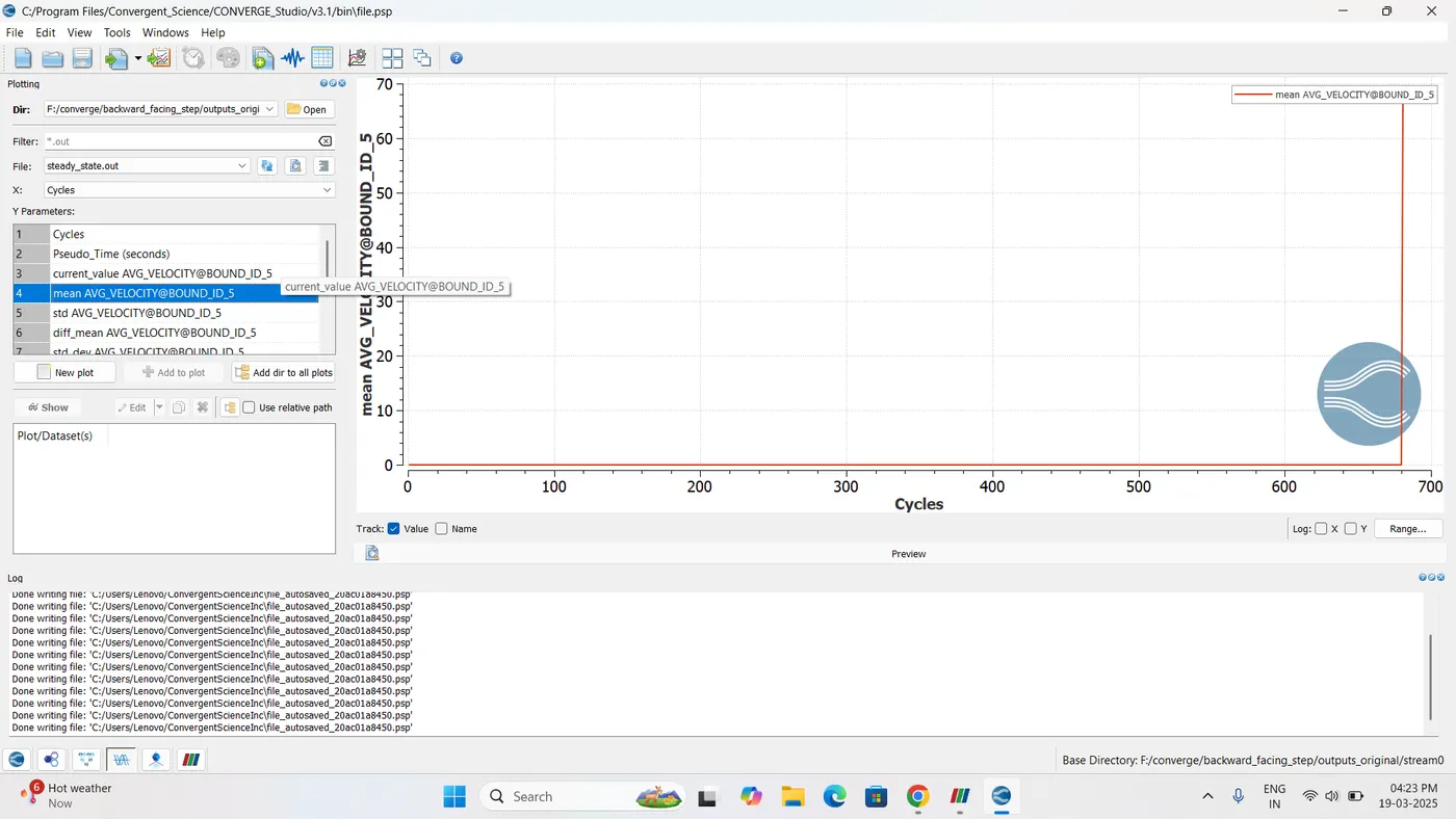
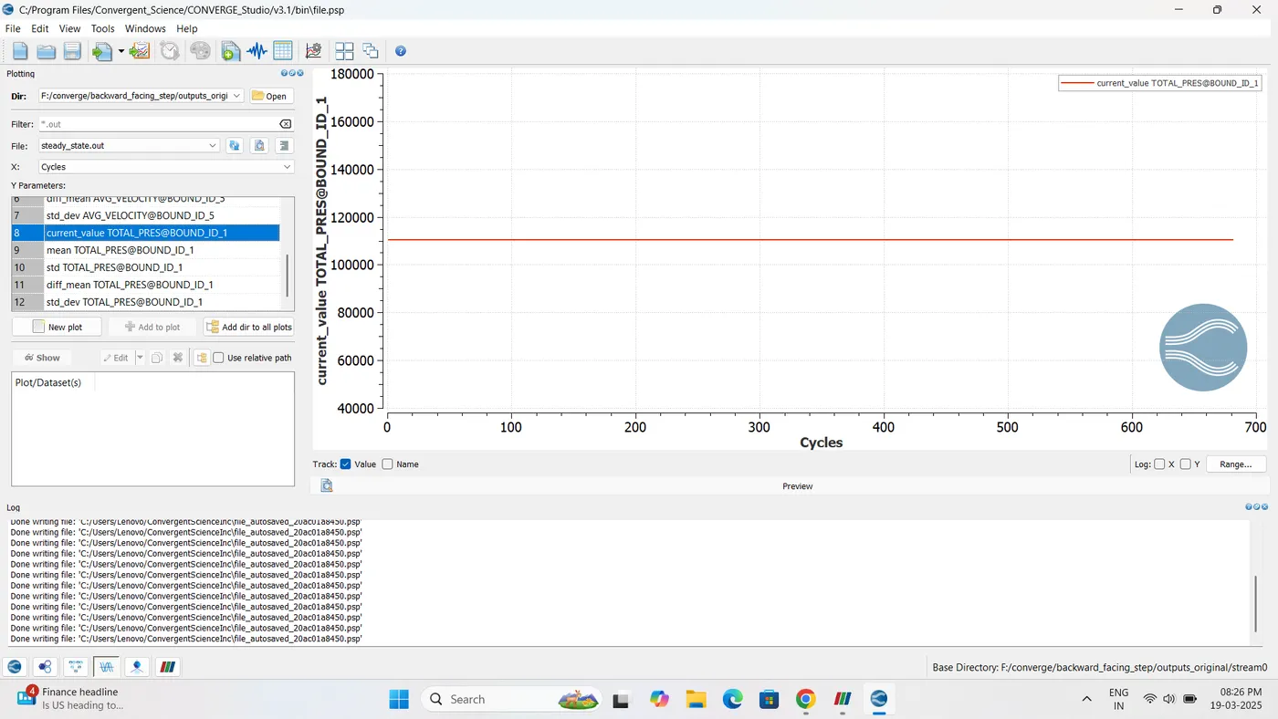
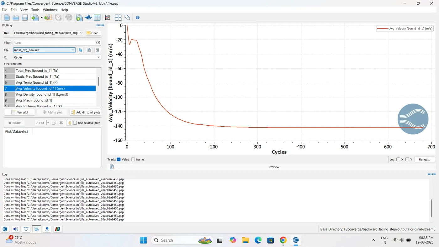
• Plot mass flow rate at the outlet

• All three bars (Coarse, Medium, Fine) should have similar height.

• Small differences are okay, but big differences mean the mesh is affecting the result.

Conclusion

The simulation of Backward Facing Step (BFS) flow was successfully carried out using CONVERGE CFD for three different mesh sizes. The results helped in understanding important flow characteristics such as flow separation, recirculation zones, vortex formation, and flow reattachment after the step.

The use of the Realisable k–ε turbulence model allowed accurate visualization of turbulent flow behavior. The simulation showed that when air hits the step, the flow separates from the wall, creating a recirculation region where eddies and vortices form. After some distance, the flow reattaches to the wall.

Key findings from the simulation include:

• Finer meshes provided better resolution of velocity and pressure contours.

• Turbulent structures were more clearly visible with finer mesh grids.

• Mass flow rate, average velocity, and pressure plots showed smoother convergence as the mesh was refined.

• Total cell count increased with mesh refinement, improving result quality but also increasing computational effort.

The flow behavior matched the expected characteristics of a turbulent separated flow:

• High velocity at the inlet, and lower velocity at the outlet due to increased cross-sectional area.

• Pressure drop near the step due to adverse pressure gradient and turbulent losses.

• Formation of vortices near the step corner and in the recirculation zone.

• Shear layer development, where the flow transitions between high and low velocities.

This study also showed the importance of mesh refinement and how it affects the accuracy and quality of simulation results. Finer meshes captured flow details better and gave smoother plots, making the analysis more reliable.

In conclusion, the BFS flow problem is an effective benchmark to study turbulence, separation, reattachment, and mesh sensitivity in CFD. The results from this simulation can be helpful in designing efficient fluid flow systems in various engineering applications like heat exchangers, diffusers, airfoils, and ventilation systems.