Week 3: Flow over a backward facing step

Flow over a backward-facing step

Objectives:

Perform a comparative study on flow over a backward facing step for the below grid configurations

• dx = dy = dz =2e-3m
• dx = dy = dz =1.5e-3m
• dx = dy = dz =1.0e-3m

Flow regimes in backward-facing step:

• Flow over a backward facing step is one of the benchmarking simulations in the field of CFD to test the codes/solvers and also a basic case to understand flow separation and recirculation.
• Initially the flow completely behaves like a channel flow and suddenly experiences a recirculation due to enlargement of section which is the backward step.
• Once the flow passes the backward step, flow separation and recirculation occurs which is explained below using several layers of flow regime.

Geometry:

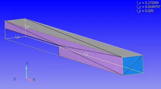
Boundary conditions:

Boundary	Condition
Inlet	Pressure 110325.0 Pa
Outlet	Pressure 101325.0 Pa
Top and Bottom faces	No slip walls
Front and Back faces	2D symmetry condition

From the boundary conditions, it is evident that the case is assumed with a symmetry boundary condition such that it is simplified numerically for faster computation with no compromise on results.

Material: The fluid across the domain is Air.

Simulation Setup:

• Steady State Simulation
• Turbulence is on - (RNG k-ε model)
• Density Based Solver is used as it is more robust in this particular tool. However, in general, pressure based solvers are used for low-speed simulations whereas density based solvers are used for high-speed flows such as flowthrough nozzles, the aerodynamics of airfoils, etc.
• Steady state is monitored based on the values mentioned in the below figure.

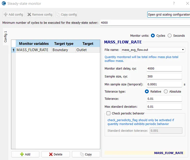
• Here, minimum number of cycles to be executed is set to 4000. The solution obtained at each iteration gets monitored only after this value of 4000 and compared whether it is below the tolerance limit. Sample Size is set to 500 cycles meaning that only if the error below the tolerance is maintained for 500 consecutive cycles, then only the computation is terminated.
• The tolerance limit and desired variables to be monitored are assigned as per computation power and desired accuracy.

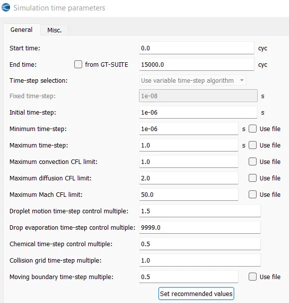
Simulation time parameters:

• Maximum number of cycles is set to 15000 but this may vary for different sizes of grids in order to achieve convergence.
• Minimum and Maximum time steps are 1e-06s and 1s respectively.
• Maximum convection CFL limit is set to 1 and Maximum diffusion CFL limit is set to 2.

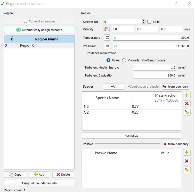
Initial conditions:

In order to initiate the numerical computation, initial conditions are defined. Here, region pressure is set equal to inlet pressure (110325 Pa), and all the boundaries are defined as a single volumetric region.

Grid Generation:

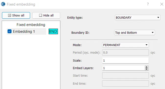
• In converge tool, the fixed embedding option is used to refine the mesh in regions where boundary layer, shocks, etc occur.
• Here, the grid is refined at the top and bottom faces in order to capture the boundary layer effectively.

Case setups and results:

Case 1: dx=2e-3m dy=2e-3m dz=2e-3m

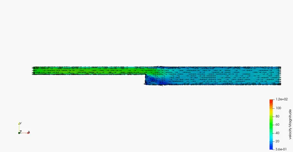
Development of Velocity contour:

Velocity contour (fully developed): (Click here)

Recirculation zone/Reattachment point:

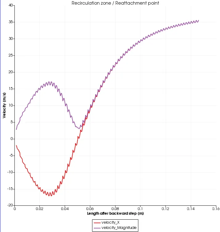
In the above plot, velocity along x is negative for a length of 0.045m. This region is the recirculation zone where the flow gets separated from the narrow channel into the broader channel. The flow which started to recirculate gets reattached to the mainstream flow which happens at 0.045m from the origin of the broader channel.

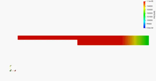
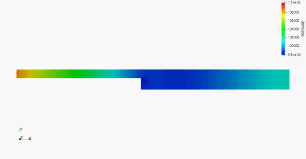
Pressure contour (fully developed): (Click here)

Case 2: dx=1.5e-3m dy=1.5e-3m dz=1.5e-3m

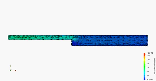
Development of Velocity contour:

Velocity contour (fully developed): (Click here)

Recirculation zone/Reattachment point:

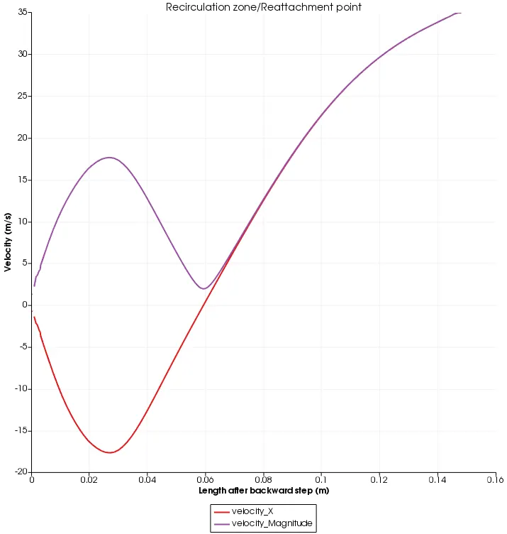
In the above plot, the reattachment point/recirculation zone has varied from the previous case. Here, reattachment length is around 0.059m.

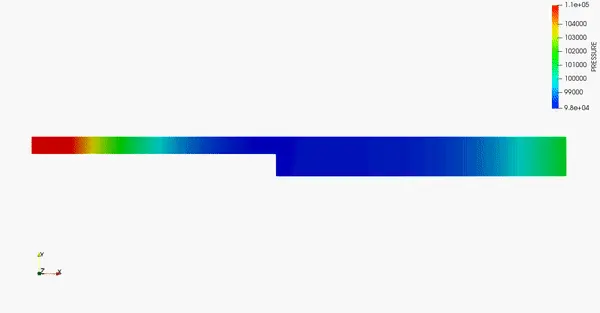
Pressure contour (fully developed): (Click here)

Case 3: dx=1e-3m dy=1e-3m dz=1e-3m

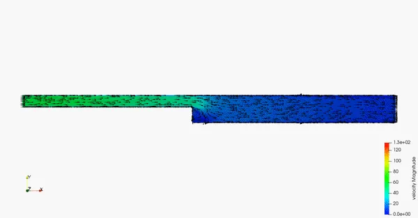
Development of Velocity contour:

Velocity contour (fully developed): (Click here)

Recirculation zone/Reattachment point:

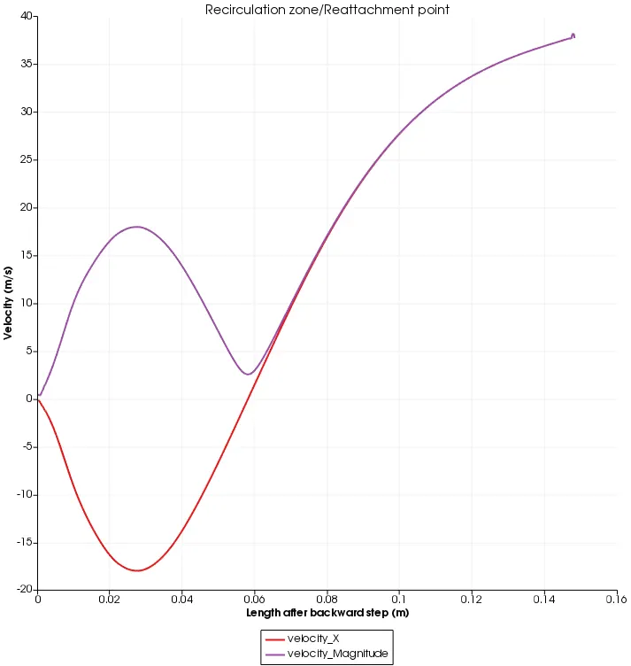
In the above plot, the reattachment point/recirculation zone has very negligible variations when compared to previous case. The reattachment length is 0.058m.

Pressure contour (fully developed):(Click here)

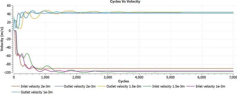
Average Velocity:

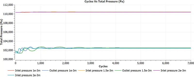
Total Pressure:

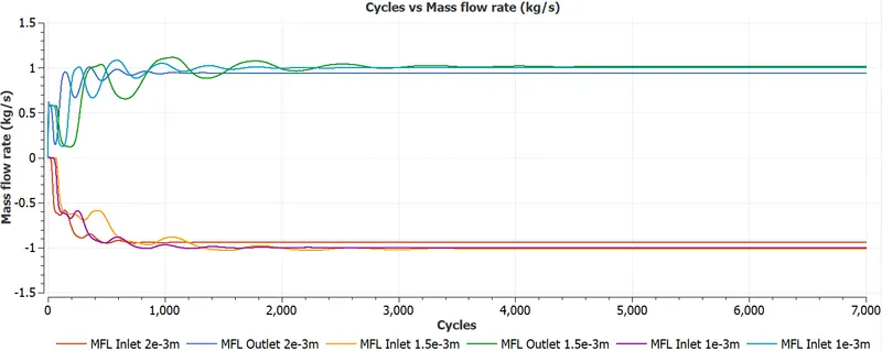
Mass flow rate:

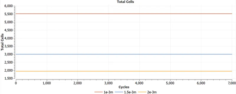
Total cells:

Inferences:

[1] Flow separation: The flow through the narrow step gets expanded at the broader step leading to separation of flow and recirculation.

[2] Reattachment Length: In the flow over backward-facing step, recirculation zone is critical. Among all cases, the case with a finer grid has around 0.058m of reattachment length.

[3] Boundary Layer: RNG k-ε Turbulence model is used to capture the boundary layer effectively.

[4] Number of cells: Case 3 has the finest grid which obviously leads to the highest number of cells.

[5] Number of Cycles: In general, the number of iterations is directly influenced by the number of cells. Higher the cells, the higher the iterations. But here the number of cycles in all 3 cases are almost similar. This may be due to the monitoring of mass conservation alone. In all cases, inlet and outlet values of pressure and velocity are nearly equal but the variation occurs inside the flow domain (Reattachment length) which is discussed in [1].