Week 3 - External flow simulation over an Ahmed body.
External flow simulation over an Ahmed body
Objective:
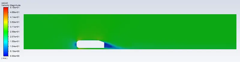
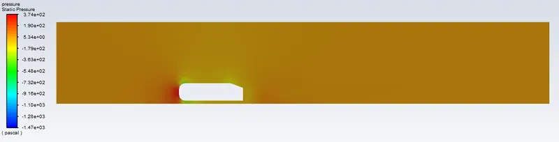
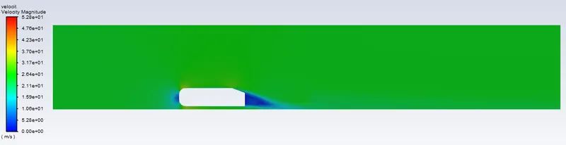
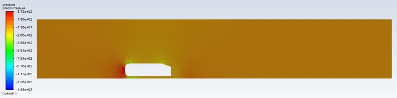
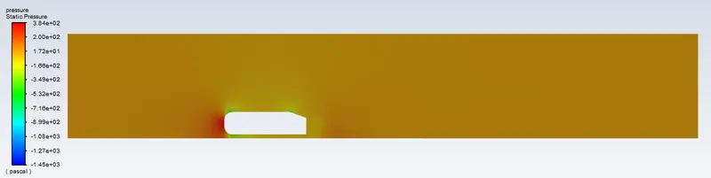
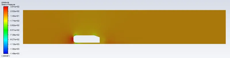
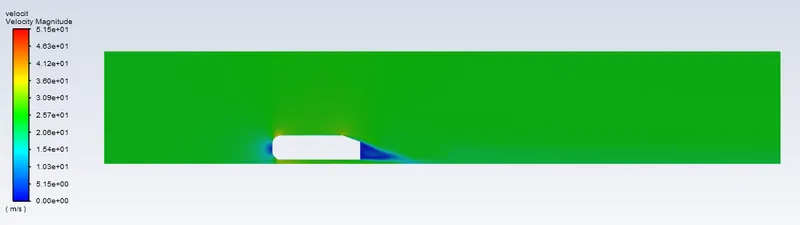
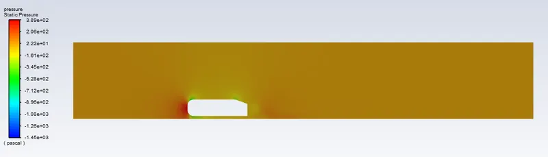
- To generate Velocity and pressure contours.
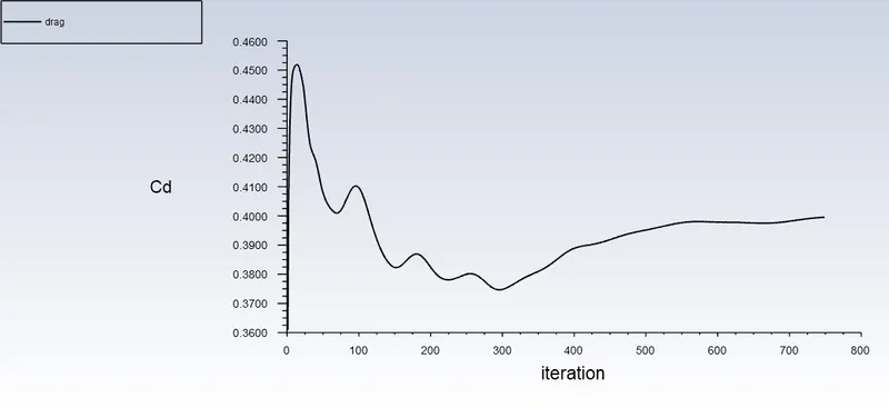
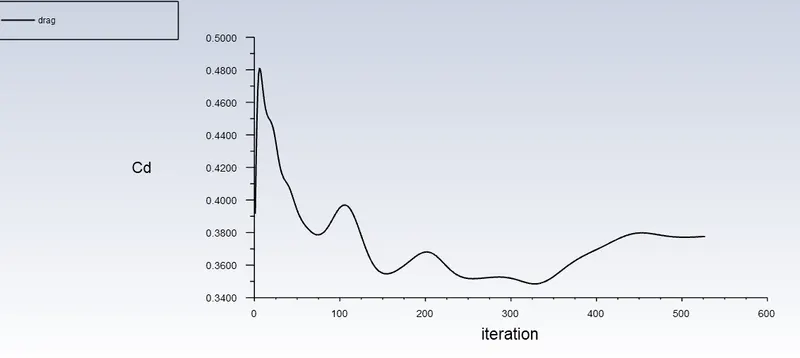
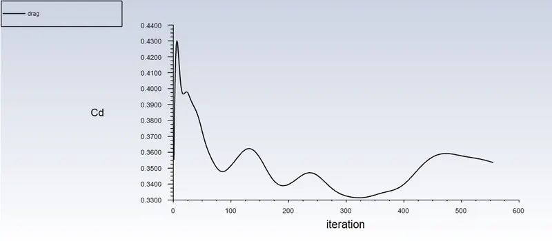
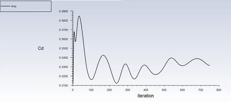
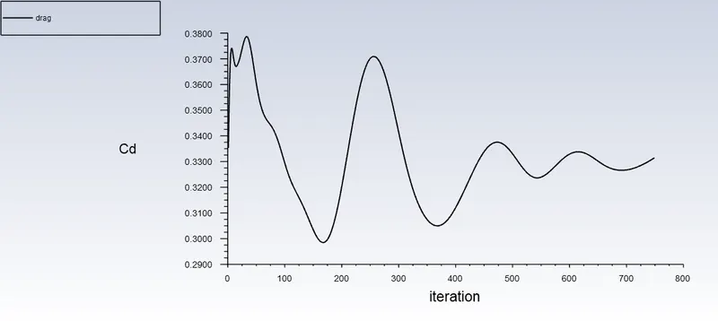
- The drag coefficient plot for a refined case. ( For velocity of 25m/sec, the drag coefficient should be around 0.33).
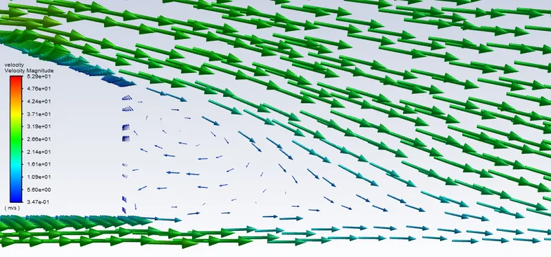
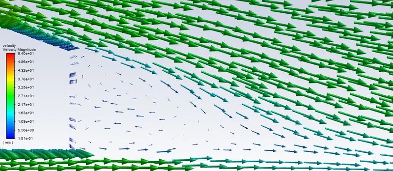
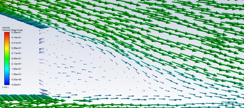
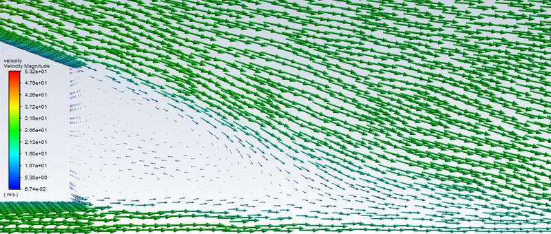
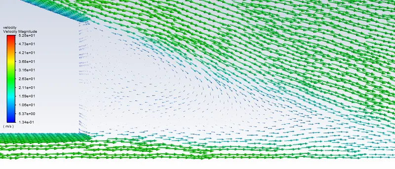
- The vector plot clearly showing the wake region.
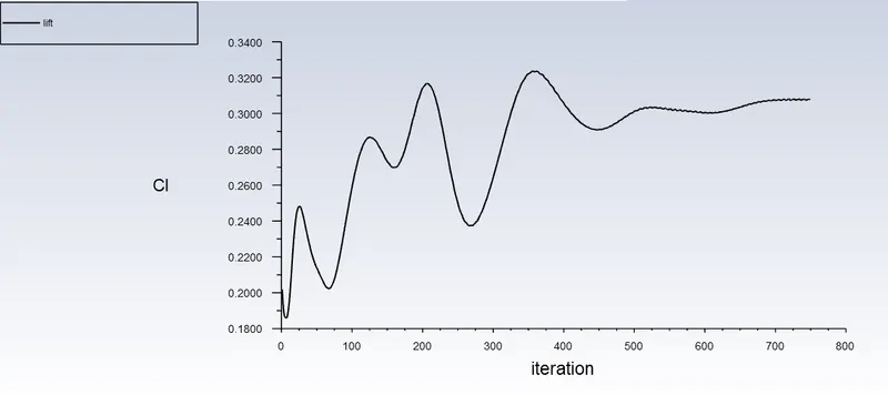
- Perform the grid independency test, provide the values of drag and lift with each case.
Ahmed Body:
- The Ahmed body is a benchmark model widely used in the automotive industry for validating simulation tools. The Ahmed body shape is simple enough to model, while maintaining car-like geometry features. It was first created by S.R. Ahmed in his research “Some Salient Features of the Time-Averaged Ground Vehicle Wake” in 1984. Since then, it has become a benchmark for aerodynamic simulation tools.
- The simple geometrical shape has a length of 1.044 meters, height of 0.288 meters, and a width of 0.389 meters. It also has 0.5-meter cylindrical legs attached to the bottom of the body and the rear surface has a slant that falls off at 40 degrees. The total drag coefficient of the Ahmed body is the key measurement for this simulation.
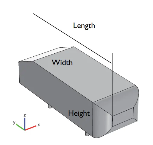
Fig. Geometry of Ahmed Body
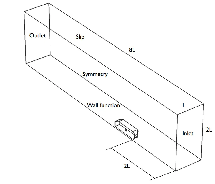
Fig. Boundary conditions and thumb rule dimensions for external flow simulations
Fig. Flow fields over Ahmed Body
In general, there are several zones and flow patterns occur over the ahmed body. Interesting zones are negative pressure in the wake region and point of separation.
Negative pressure in the wake region:
The wake is the region of disturbed flow (often turbulent) downstream of a solid body moving through a fluid, caused by the flow of the fluid around the body. In Ahmed Body, it is the region behind the back end of the body. They are also further subdivided into near wake, far wake region based upon the distance from the end of solid body.
The pressure gradient is the horizontal change in pressure divided by the horizontal change in distance. Whenever the pressure gradient is negative, it accelereates the flow overcoming the viscous forces. Hence a negative pressure gradient is termed a Favourable pressure gradient. On the other hand, a positive pressure gradient has the opposite effect and is termed the Adverse Pressure Gradient. This adverse pressure gradient is the reason behind the negative pressure in the wake region.
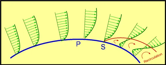
Fig. Separation of flow over a curved surface
One of the severe effects of an adverse pressure gradient is to separate the flow. Consider flow past a curved surface as shown in Fig. The geometry of the surface is such that we have a favourable gradient in pressure to start with and up to a point P. The negative pressure gradient will counteract the retarding effect of the shear stress (which is due to viscosity) in the boundary layer. For the geometry considered we have a an adverse pressure gradient downstream of P.
Now the adverse pressure gradient begins to retard. This effect is felt more strongly in the regions close to the wall where the momentum is lower than in the regions near the free stream. As indicated in the figure, the velocity near the wall reduces and the boundary layer thickens. A continuous retardation of flow brings the wall shear stress at the point S on the wall to zero. From this point onwards the shear stress becomes negative and the flow reverses and a region of recirculating flow develops. We see that the flow no longer follows the contour of the body. We say that the flow has separated. The point S where the shear stress is zero is called the Point of Separation.
Baseline Setup:
Geometry:
The Ahmed Body is enclosed using an enclosure by providing more area for the wake region so as to visualise the complete recirculation.
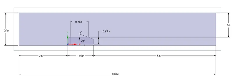
Fig. Baseline geometry
Meshing:
Initially for setting up the entire case, a baseline mesh is created.
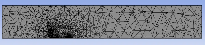
Fig. Baseline Mesh-Nodes: 16598, Elements: 84094, Element size: 0.4136 m
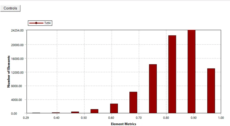
Mesh Quality is as follows. All the elements are tetra and the quality is not sufficient for the problem which is being solved.
Case Setup:
- Steady State Simulation
- Turbulence on, Viscous model-k epsilon
- Solver-Density based
Boundary Conditions:
- Velocity Inlet: 25 m/s
- Pressure Outlet: 0 Gauge Pressure
- Wall : Ahmed Body
- Symmetry: Enclosure walls
Working Fluid: Air
Output Plots: (Iterations 200)
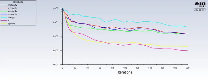
Residual Plot:
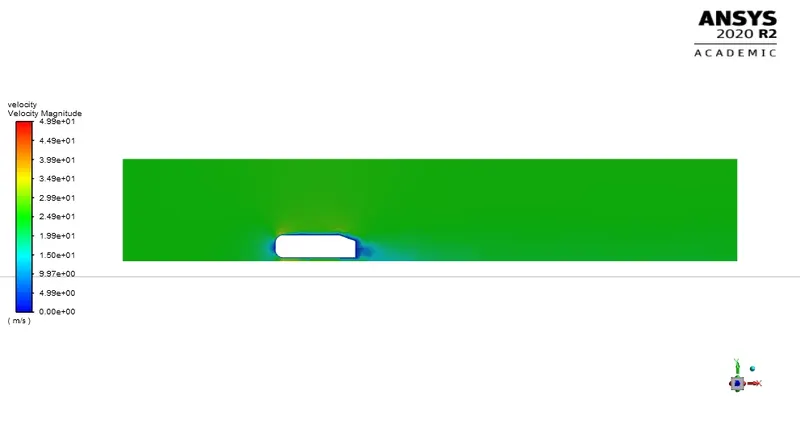
Velocity Plot:
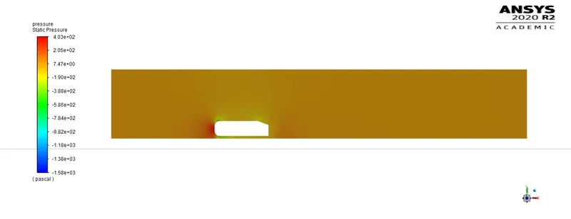
Pressure Plot:
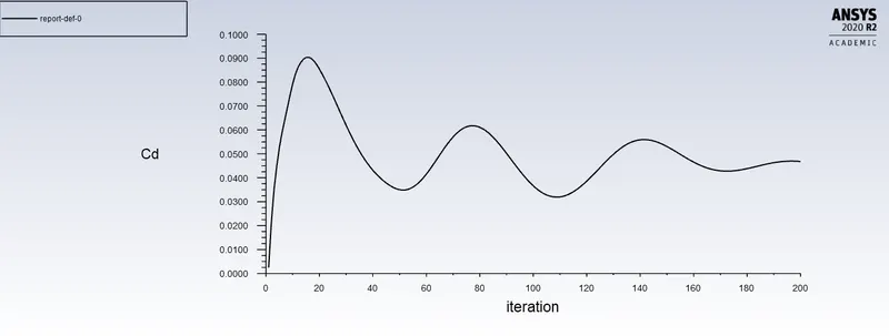
Coefficient of Drag:
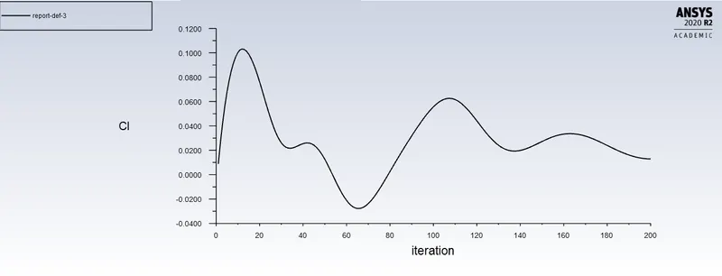
Coefficient of Lift:
Inferences:
- Velocity and Pressure Plots clearly shows that the recirculation region is not well distinguished. This is due to coarse mesh.
- Cd is around 0.05, which is a huge deviation from literature results of 0.33.
Refined Setup:
Geometry:
In the geometry, an additional enclosure surrounding the ahmed body has been added to capture the near wake region flow recirculation.
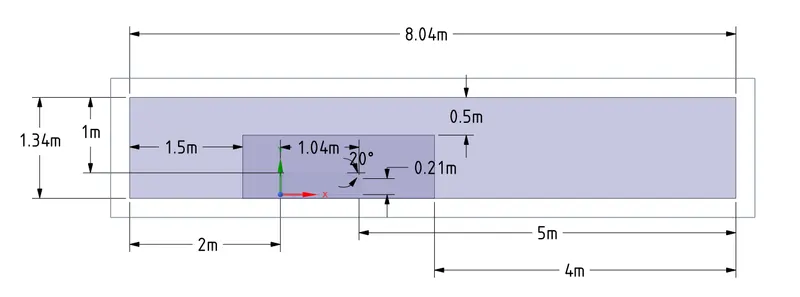
Fig. Refined Geometry
Meshing:
Refined mesh consists of 5 Stages.
1. Baseline Mesh with element size 0.12m
2. Multizone Mesh with Hexa Elements at the outermost enclosure (Baseline enclosure).
3. Bodysizing the inner enclosure with element size of 0.05m (Refined case enclosure).
4. Face sizing on Ahmed Body faces with element size 0.01 m.
5. Adjustment of Inflation layer to capture the boundary layer accurately.
Estimation of first cell thickness:
Value of  is to distinguish different regions near the wall / viscous region. Let us try to understand this with an example. A fisherman uses fishing net, a grid kind of structure to trap the fishes. If he is trying to catch medium to big sized fishes the grids in the net he uses is somewhat big, but if he is trying to trap even small sized fishes then the grid size of the net should be small enough to capture them. In this case even the large fishes are also captured. Similarly coming back to our case if we intend to resolve the effects near the wall i.e., in the viscous sub layer then the size of the mesh size should be small and dense enough near the wall so that almost all the effects are captured.This is ideal to get the correct estimation of drag and lift forces.
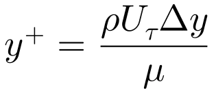
where  is shear velocity, ρ - density (kg/m3) and μ is kinematic viscosity (kg/m-s) and target value is estimated based on the turbulence model used.
- First lets calculate the reynolds number,
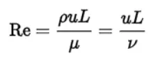
Re = (1.225*25*1.04)/0.000017894 = 17,79,926.23 (Turbulent Flow)
- Skin Friction Coefficient for external flows is,

Cf = 0.0032609
- Wall shear stress ,
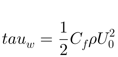
tau = 0.5*0.0032609*1.225*25*25 = 1.248 kg /m-s^2
Here Uo is free stream velocity = 25 m/s
- Shear Velocity
Shear velocity, Ut = 1.009 m/s
- Now finally to calculate first cell thickness, △y
y+ can be > 30, (Since k-ε is the turbulence model due to high reynolds number)
First cell thickness, △y= 7.2385267288283003984547238122206e-4 m (Here y+ = 50)
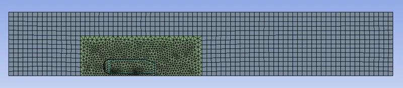
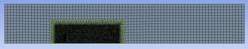
Fig.Refined Mesh
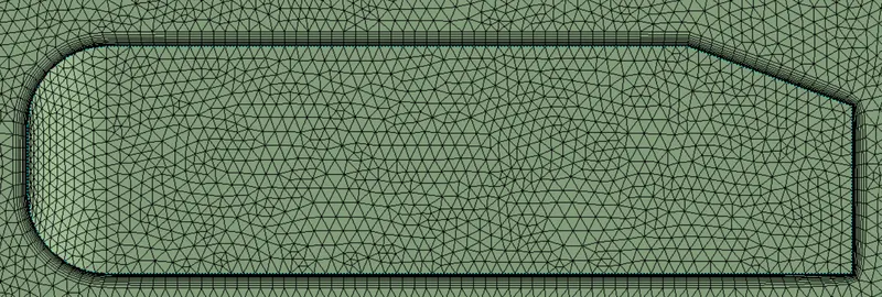
The below figure shows the near wall region of ahmed body which is given a inflation layer of 10 with above calculated first cell thickness.
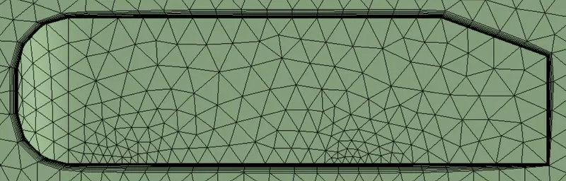
Fig. Inflation Layer near wall
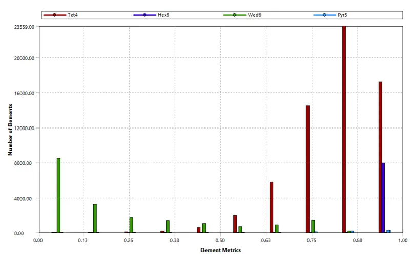
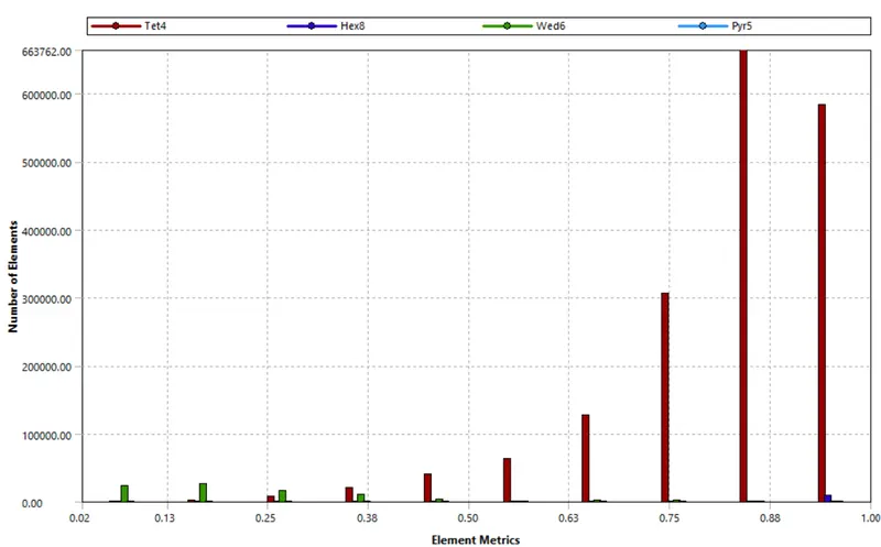
Fig. Mesh Quality
Case Setup:
- Steady State Simulation
- Turbulence on, Viscous model: k-ε (In order to capture near wall field accurately)
- Solver-Density based
Boundary Conditions:
- Velocity Inlet: 25 m/s
- Pressure Outlet: 0 Gauge Pressure
- Wall : Ahmed Body
- Symmetry: Enclosure walls
Working Fluid: Air
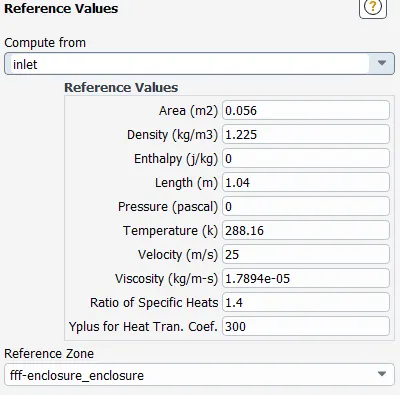
Reference Values:
Result:
Grid Independence Test:
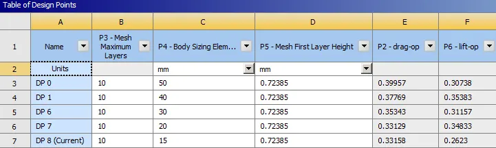
This test is performed by varying the body size elements around the ahmed body from 50mm to 15mm. Finally grid independence has been achieved at 15mm with a drag coefficient of 0.33.
Output Plots at case 1 (DP 0):
Residual Plot:
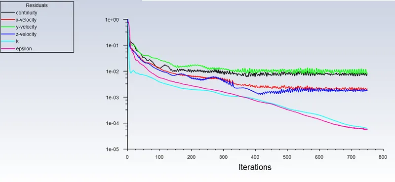
Velocity Contour:
Velocity vector plot at the wake region(recirculation zone):
Pressure Contour:
Drag Coefficient Plot:
Lift Coefficient Plot:
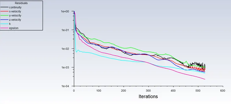
Output Plots at case 2 (DP 1):
Residual Plot:
Velocity contour:
Velocity vector plot at the wake region(recirculation zone):
Pressure contour:
Drag Coefficient Plot:
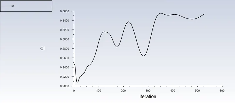
Lift Coefficient Plot:
Output Plots at case 3 (DP 6):
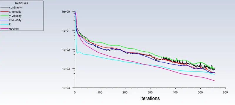
Residual Plot:
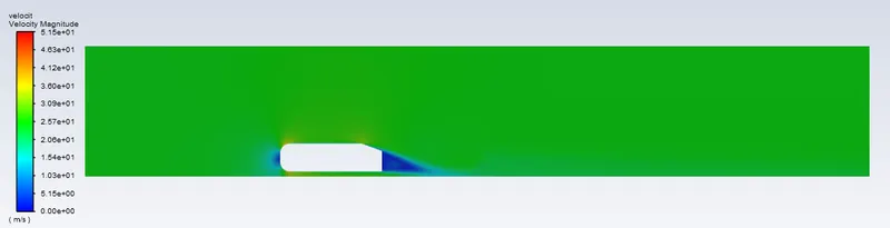
Velocity contour:
Velocity vector plot at the wake region(recirculation zone):
Pressure contour:
Drag Coefficient Plot:
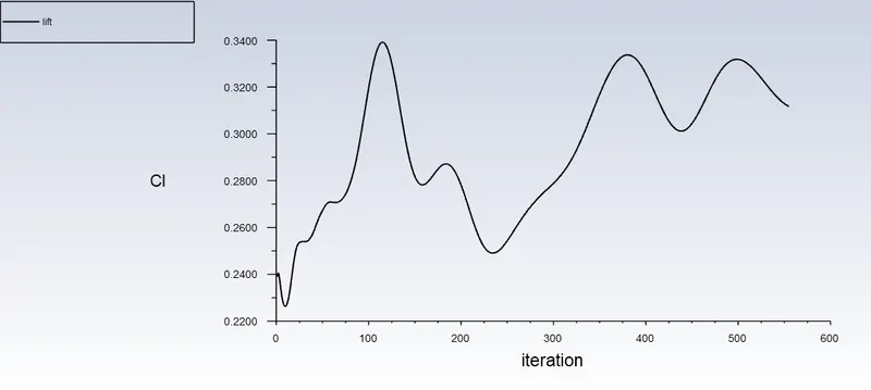
Lift Coefficient Plot:
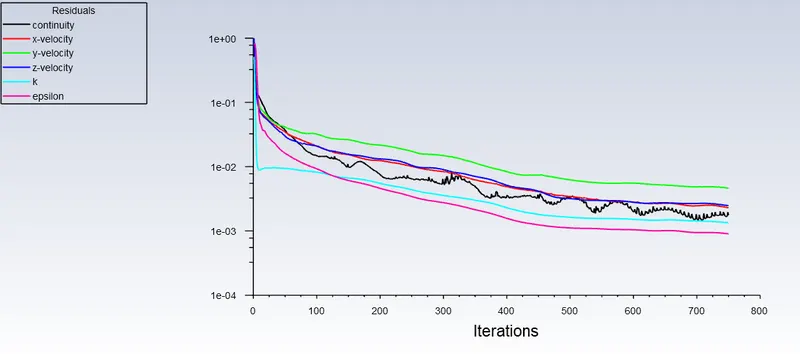
Output Plots at case 4 (DP 7):
Residual Plot:
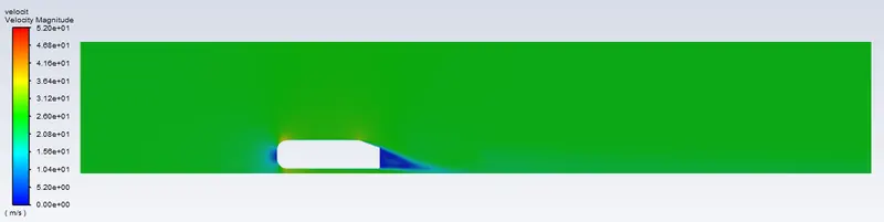
Velocity contour:
Velocity vector plot at the wake region(recirculation zone):
Pressure contour:
Drag Coefficient Plot:
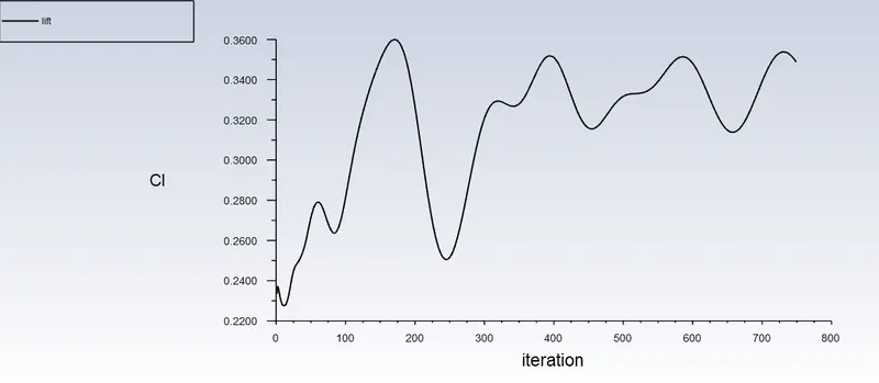
Lift Coefficient Plot:
Output Plots at case 5 (DP 8):
- Below are the mesh and its quality at 0.33 of Cd.
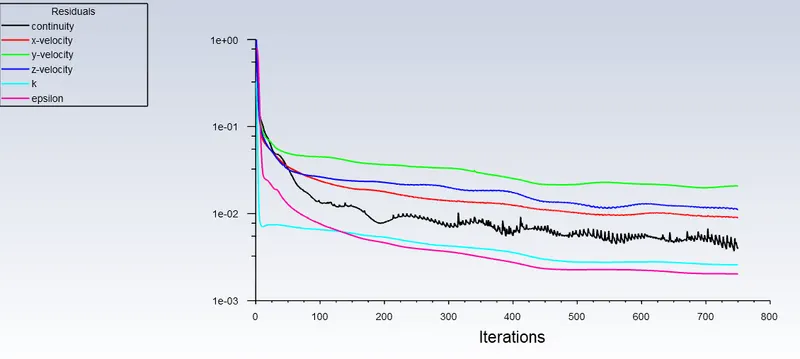
Residual Plot:
Velocity Contour:
Velocity vector plot at the wake region(recirculation zone):
Pressure Contour:
Drag Coefficient Plot:
Lift Coefficient Plot:
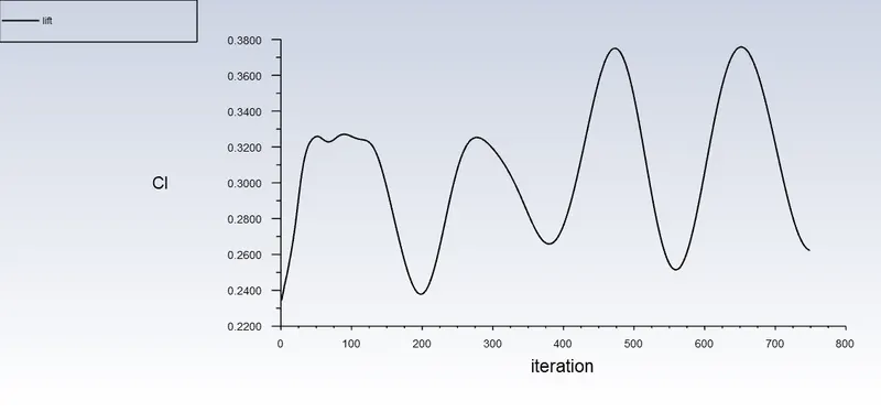
Inferences:

At Design Point 8, Drag coefficient (Cd) of 0.33 has been achieved.
References:
1. https://www.computationalfluiddynamics.com.au/tips-tricks-cfd-estimate-first-cell-height/
3. CFD Aerodynamic Analysis of Ahmed Body, Rehan Salahuddin Khan1, Sudhakar Umale2, International Journal of Engineering Trends and Technology (IJETT).