Week 3 - External flow simulation over an Ahmed body.

AIM-:
Study of Flow and Turbulence Structures in the Wake of a Simplified Car Model (Ahmed Model)

Theory-:
Ahmed Body

                                            
The Ahmed body is a generic car body (a simplified vehicle model). The airflow around the Ahmed body captures the essential flow features around an automobile and was first defined and characterized in the experimental work of Ahmed . Although it has a very simple shape, Ahmed body allows us to capture characteristic features that are relevant to bodies in the automobile industry. This model is also used to describe the turbulent flow field around a car-like geometry. Once the numerical model in validated, it is used to design new models of the car. The rear part of Ahmed body called as 'slant angle' which influences drag and lift with its critical slant angle which is around 0-30 degree.
Importance of Ahmed Body
1. Ahmed Body plays a vital role in testing the aerodynamic properties of vehicle.
2. It is also used to describe the turbulent flow field around a car-like geometry and later to design new car models with validated results.

Boundary Layers with Pressure Gradients

FIGURE-1

                                                                                                                 

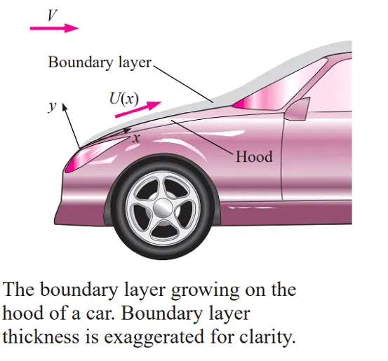
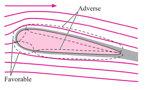
When the flow in the inviscid and/or irrotational outer flow region (outside of the boundary layer) accelerates, U(x) increases and P(x) decreases. We refer to this as a favorable pressure gradient. It is favorable or desirable because the boundary layer in such an accelerating flow is usually thin, hugs closely to the wall, and therefore is not likely to separate from the wall. When the outer flow decelerates, U(x) decreases, P(x) increases, and we have an unfavorable or adverse pressure gradient. As its name implies, this condition is not desirable because the boundary layer is usually thicker, does not hug closely to the wall, and is much more likely to separate from the wall. In a typical external flow, such as flow over an airplane wing (Fig- 2), the boundary layer in the front portion of the body is subjected to a favorable pressure gradient, while that in the rear portion is subjected to an adverse pressure gradient. If the adverse pressure gradient is strong enough (dpdx)≥0">(dpdx)≥0(����)≥0 ,the boundary layer is likely to separate off the wall. Examples of flow separation are shown in figure-1 for external flows. The figure is sketched an airfoil at a moderate angle of attack. The boundary layer remains attached over the entire lower surface of the airfoil, but it separates somewhere near the rear of the upper surface as sketched. The closed streamline indicates a region of recirculating flow called a separation bubble. As pointed out previously, the boundary layer equations are parabolic, meaning that no information can be passed from the downstream boundary. However, separation leads to reverse flow near the wall, destroying the parabolic nature of the flow field, and rendering the boundary layer equations inapplicable.

FIGURE-2

                                                                                                             

N.B-: The boundary layer equations are not valid downstream of a separation point because of reverse flow in the separation bubble.

In the above cases, the full Navier–Stokes equations must be used in place of the boundary layer approximation. From the point of view of the boundary layer procedure , the procedure breaks down because the outer flow no longer valid when separation occurs, especially beyond the separation point . Figure-3 shows the classic case of an airfoil at too high of an angle of attack, in which the separation point moves near the front of the airfoil; the separation bubble covers nearly the entire upper surface of the airfoil—a condition known as stall. 

FIGURE-3

                                                                                                   

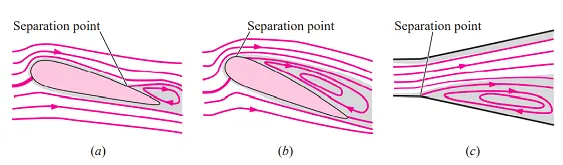
Stall is accompanied by a loss of lift and a marked increase in aerodynamic drag.

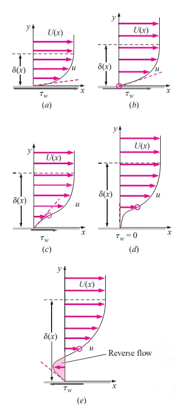
Since the velocity is zero at the wall (no-slip condition), the entire left side of Navier-stokes equation disappears, leaving only the pressure gradient term and the viscous term, which must balance, At the wall Under favorable pressure gradient conditions (accelerating outer flow), dU/dx is positive, and , (del^2u)/(dely^2) in N-S equation at the wall is negative. We know that (del^2u)/(dely^2) must remain negative as u approaches U(x) at the edge of the boundary layer. Thus, we expect

1. the velocity profile across the boundary layer to be rounded, without any inflection point, as sketched in Fig.-4 (a).

2. Under zero pressure gradient conditions, implying a linear growth of u with respect to y near the wall, as sketched in Fig-4 (b).

3. For adverse pressure gradients, dU/dx is negative and N-S equation demands that ∂2u∂y2">∂2u∂y2∂2�∂�2 be positive. However, since it must be negative as u approaches U(x) at the edge of the boundary layer, there has to be an inflection point somewhere in the boundary layer, as illustrated in Fig-4 (c.)

The first derivative of u with respect to y at the wall is directly proportional to τw">τw��, the wall shear stressτw=μ(∂u∂y)">τw=μ(∂u∂y)��=�(∂�∂�). Comparison of ∂u∂y">∂u∂y∂�∂� in Fig-4 (a) through c reveals that shear stress is largest for favorable pressure gradients and smallest for adverse pressure gradients. Boundary layer thickness increases as the pressure gradient changes sign, as also illustrated in Fig-4. If the adverse pressure gradient is large enough,∂u∂y">∂u∂y∂�∂� can become zero (Fig-4 (d)); this location along a wall is the separation point, beyond which there is reverse flow and a separation bubble (Fig-4 e). Notice that beyond the separation point τw">τw�� is negative due to the negative value of ∂u∂y∣0">∂u∂y∣∣∣0∂�∂�∣0. As mentioned previously, the boundary layer equations break down in regions of reverse flow. Thus, the boundary layer approximation may be appropriate up to the separation point, but not beyond.

FIGURE-4

                                                                                                                                  

N.B- We use computational fluid dynamics (CFD) to illustrate flow separation for the case of flow over a bump along a wall. (AHMED BODY)

CFD CASE SET UP AND SIMULATION

First we need to start the workbench and select fluid flow (fluent) solver. Then setup the steps shown in fluent solver as follows.

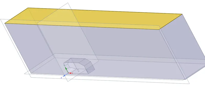
Geometry :

1. Open the Geometry.

2. Import the Ahmed Body.

5. Split the body into half.

3. Provide Enclosures to ahmed body (Inner and outer) according to given dimensions.

4. Suppress the Ahmed body.

5. This completes the geometry step.

The dimensions used are:

                                                                                      

Mesh :

1. Start the mesh section.

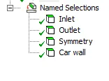
2. Name the boundaries, which are Inlet, Outlet, Symmetry, Wall, Car-wall.

                                                                                   

3. Then, provide specific element size and generate the mesh.

                                       

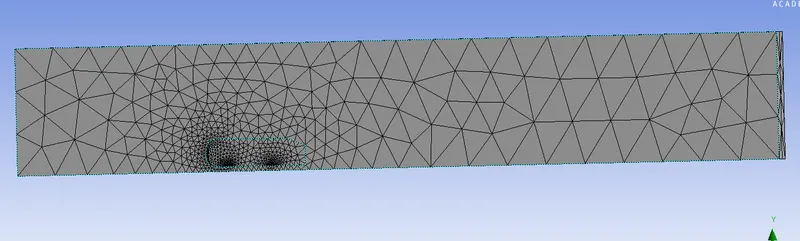
                                        (Base line mesh)

The quality of mesh used is good as the least quality is above 0.1

Setup :

                                                                                     

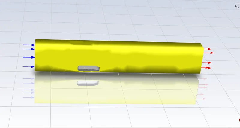
1. First, we need to check the mesh from Domain section.

2. secondly, check if the boundaries hve been specified correctly.

3. Now, provide the reference values according to the problem.

4. set the turbulence model (K-OMEGA (SST)).

5. Select the solver (simple taken by default setting) according to the problem.

6. Now, set in the boundary conditions like inlet velocity, guage pressure, etc.

Inlet velocity- 5 m/sec

outlet- gauge pressure = 0 pa

car wall- No sleep

7. In solution section create drag and lift reports and plots, also set the solution method.

8. Now, go to the results section and create a plane at some distance normal to x,y,z axis which will be used to examine the velocity and pressure along it.

9. Initialize the problem with Hybrid Initialization.

10. Go back to result section and add velocity and pressure contours along plane. Also add velocity animation.

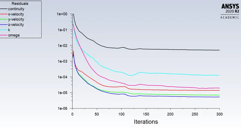
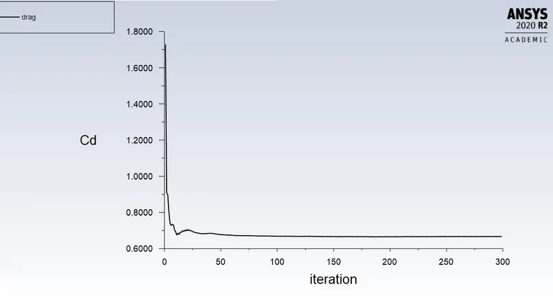
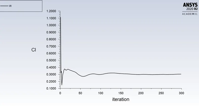
11. Finally simulate the problem for some amount of iteration and ovserve the Drag, Lift and Residual plots.

12. This completes the setup section.

RESIDUAL

                                                                     

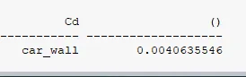
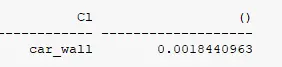
Drag co-efficient

                                                                                                                             

                                                                                                        

Lift co-efficient

                                                                                          

                                                                                          

Results :

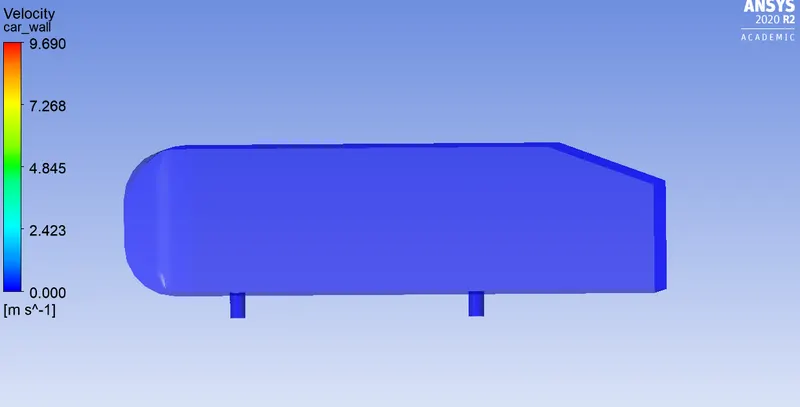
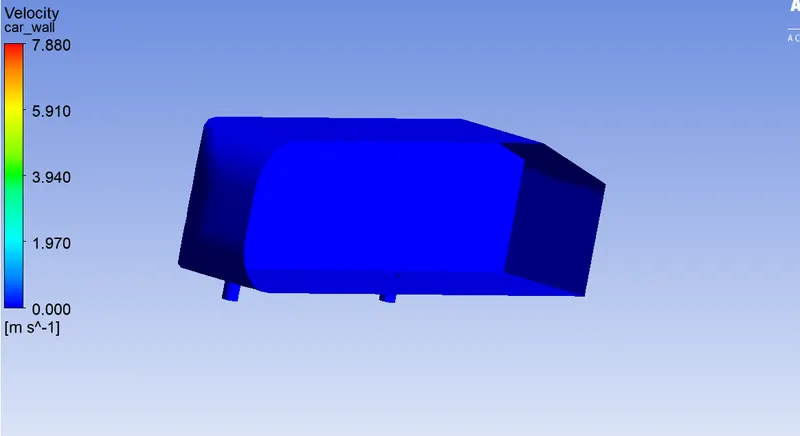
1. Select the wall volume to make it visible. Also color it with the variable needed to be observed.

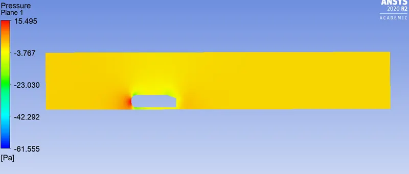
2. After that, insert the plane and color it with variable like Pressure and Velocity which shows the Pressure and Velocity flow on plane.

3. Edit the legend according to requirement. This completes the results and hence the entire simulation.

                                                 

                                                

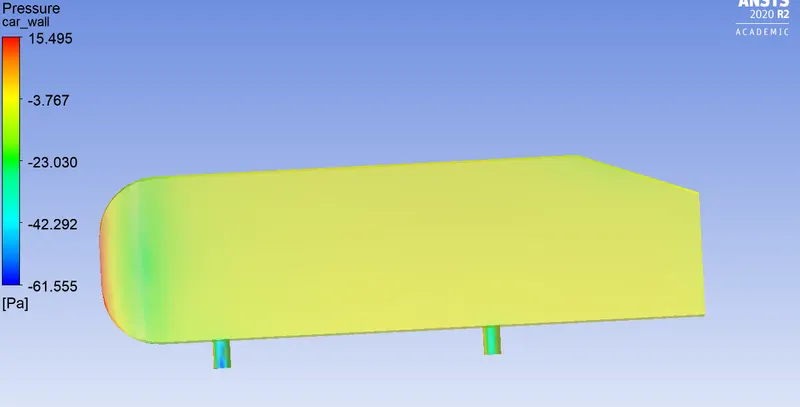
PRESSURE

 

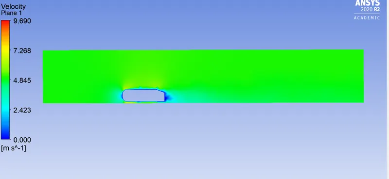
VELOCITY

                                                

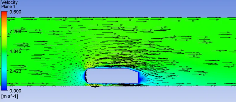
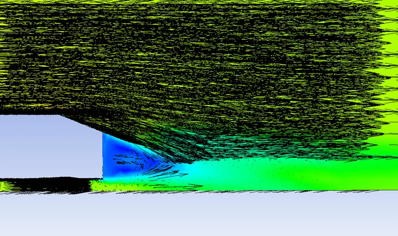
VECTOR PLOT- VELOCITY

                                          

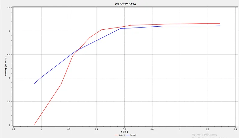
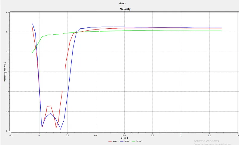
VELOCITY DATA AT (X,Y) = (1.5,2) AND (2,2)

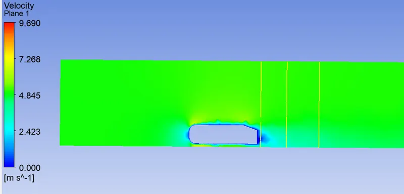
In case-2 We will be performing a refined case with Y+ 

CASE-2

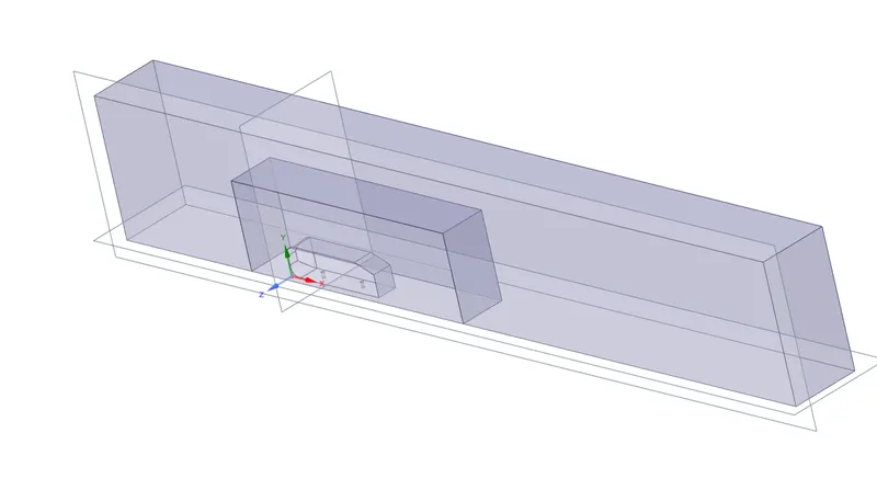
1. Open the Geometry.

2. Import the Ahmed Body.

5. Split the body into half.

3. Provide Enclosures to ahmed body (Inner and outer) according to given dimensions.

4. Suppress the Ahmed body.

 5. Input Planes & select XY plane and view the interference range.

6. Now, go to prepare and check for interference and correct it.

7. Set the topology to share.

5. This completes the geometry step.

                                                                      

Mesh

1. Start the mesh section.

2. Name the boundaries, which are Inlet, Outlet, Symmetry, Wall, Car-wall.

                                                                                   

3. Then, provide specific element size and generate the mesh.

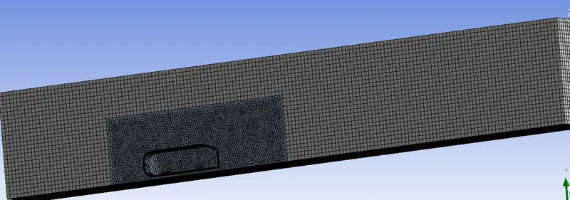
4. Then, we have to provide the mesh method for the outer enclosure & set the multizone method so it creates Hexagonal mesh elements over that enclosure.

5. Then, we have to add Body sizing for the inner enclosure to make it more refined in inner bounding box.

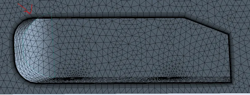
6. Now, add face sizing to the legs of ahmed body so they become completly circular (no sharp corner ), while making their mesh element size shoud be smaller (5mm taken in our case).

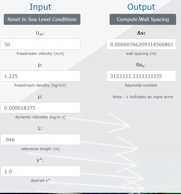
7. Finally, add inflation layers according to correct y+ values.

                                                                                                   

8. This completes Mesh section.

                                            

                                               

Setup :

                                                                                     

1. First, we need to check the mesh from Domain section.

2. secondly, check if the boundaries hve been specified correctly.

3. Now, provide the reference values according to the problem.

4. set the turbulence model (K-OMEGA (SST)).

5. Select the solver (simple taken by default setting) according to the problem.

6. Now, set in the boundary conditions like inlet velocity, guage pressure, etc.

Inlet velocity- 5 m/sec

outlet- gauge pressure = 0 pa

car wall- No sleep

7. In solution section create drag and lift reports and plots, also set the solution method.

8. Now, go to the results section and create a plane at some distance normal to x,y,z axis which will be used to examine the velocity and pressure along it.

9. Initialize the problem with Hybrid Initialization.

10. Go back to result section and add velocity and pressure contours along plane. Also add velocity animation.

11. Finally simulate the problem for some amount of iteration and ovserve the Drag, Lift and Residual plots.

12. This completes the setup section.

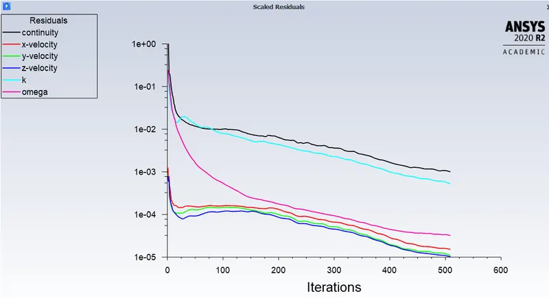
RESIDUAL

                                                     

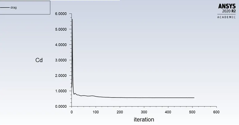
Drag co-efficient

                                                   

                                                 

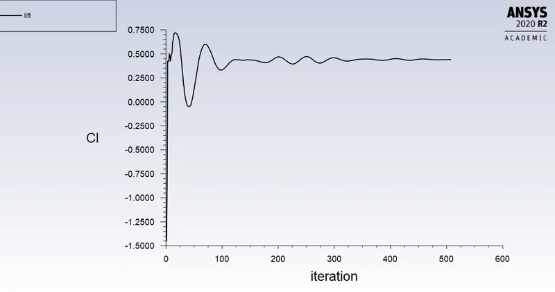
LIFT co-efficient

                                                 

                                               

Results :

1. Select the wall volume to make it visible. Also color it with the variable needed to be observed.

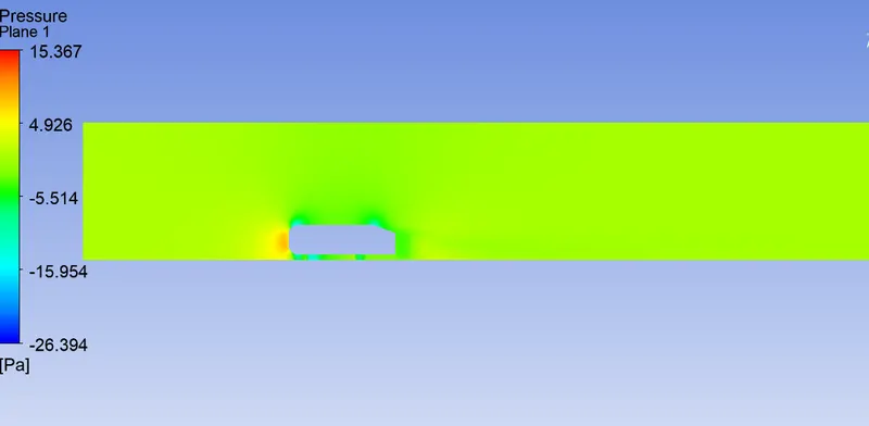
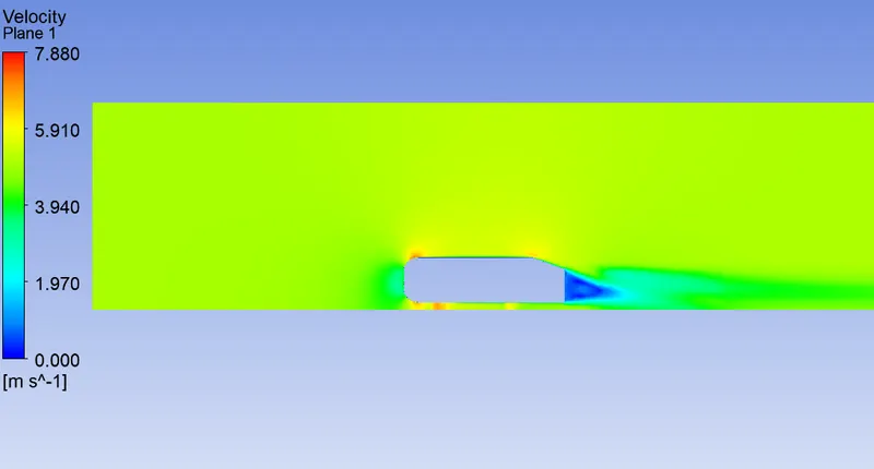
2. After that, insert the plane and color it with variable like Pressure and Velocity which shows the Pressure and Velocity flow on plane.

3. Edit the legend according to requirement. This completes the results and hence the entire simulation.

                                               

                                               

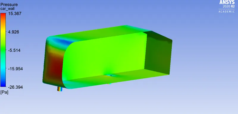
PRESSURE

VELOCITY

                                               

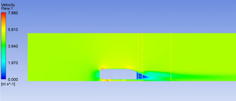
VELOCITY DATA

                                       

                                     

VECTOR PLOT- VELOCITY

CONCLUSIOn

1.We compare the CFD results to experimental results. The calculated time-averaged drag and lift coefficient on the Ahmed body is .34 and     respectively. As mentioned previously, experimental values of C_D at this Reynolds number is .33, so the agreement is nearly matches with the experimental scatter by mesh refinement and good choice of Y+ value.

2. We use computational fluid dynamics (CFD) to illustrate flow separation for the case of flow over a bump (Ahmed body) along a wall. The flow is steady and twodimensional and vector plot shows outer flow velocity vector generated by a solution of the Navier-Stokes equation.

3. When the full (laminar) Navier–Stokes equation is solved, the viscous terms lead to flow separation off the rear end of the bump, as seen in vector plot.

4. The approximate location of the separation point is indicated in vector plot, and the dashed black line is a type of dividing streamline. Fluid below this streamline is caught in the separation bubble, while fluid above this streamline continues downstream.

5. In the vector plot Reverse flow in the lower portion of the separation bubble is clearly visible. Also, there is a strong y-component of velocity beyond the separation point, and the outer flow is no longer nearly parallel to the wall. In fact, the separated outer flow is nothing like the original outer flow. This is typical and represents a serious deficiency in the boundary layer approach.

 References

1. G. T. Yates. “How Microorganisms Move through Water,” American Scientist, 74, pp. 358–365, July–August, 1986.

2. R. J. Heinsohn and J. M. Cimbala. Indoor Air Quality Engineering. New York: Marcel-Dekker, 2003.

3. P. K. Kundu. Fluid Mechanics. San Diego, CA: Academic Press, 1990.