Mobile Drop test using LS-Dyna Explicit Solver

AIM: To set up the solver deck file for the Mobile drop case.

ABSTRACT: In this assignment, we are going to study the case of the mobile drop situation. This will be done by setting up the keyword necessary to mimic the actual condition. we will also assign the initial velocity card and set boundary conditions and extract results from the output files(D3plots & ASCII files)

METHODOLOGY: We need to follow a few steps to set up the deck file.

1. Import the model (.K file)as LS Dyna keyword file
2. Build the material card for mobile and ground
3. Create the section card for the mobile and ground
4. Create the part card for the mobile and ground link the material card and section card to it
5. Create a contact interface between mobile and ground surface to the surface [set master and slave]
6. Give the initial velocity towards the ground direction
7. Create the boundary condition for arresting the DOF of the plate.
8. Set up the termination card, control cards, and tile.
9. Run the model check and see for any errors.
10. Save the file as Ls Dyna keyword file.
11. Run the file in the LS RUN and see the D3PLOTS (animations)

PROCEDURE:

we are following the unit system as[ gram, millimeter, millisecond]

Import the model (.K file)as LS Dyna keyword file

once we import the file we can see there are three parts 2 solid(green and yellow) and 1 shell(red). We need only a solid mobile(green) and shell ground(red). so we need to delete the yellow solid part, so as to proceed further.

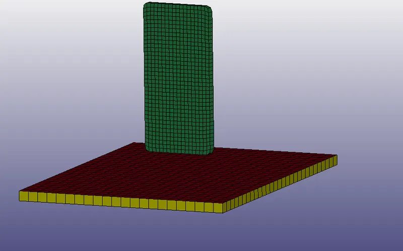
Fig 1. Imported file

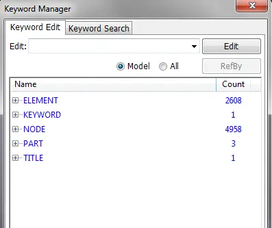
Fig.2 imported keyword manager

so to delete that we can go to the keyword >part> delete the yellow part>accept>done

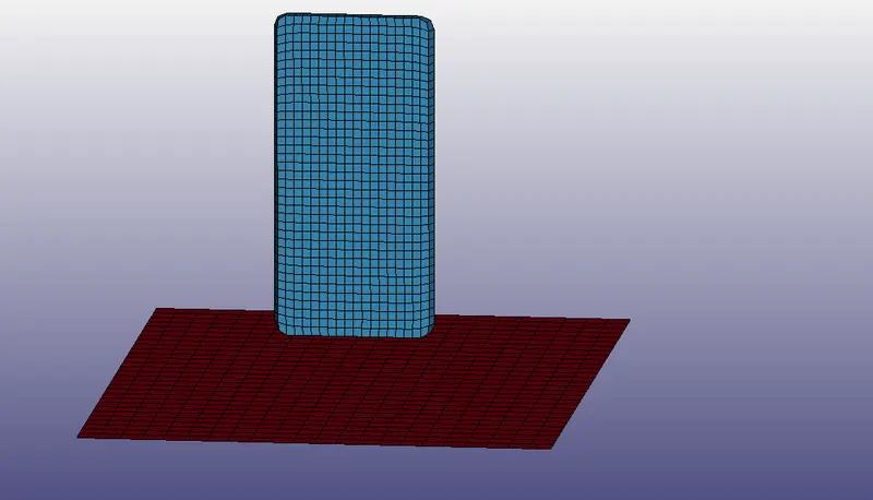
Fig.3 Required mobile and ground model

Build the material card for mobile and ground

Once we get the required meshed model we will set the material card for both the parts i.e mobile and ground.

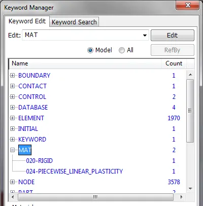
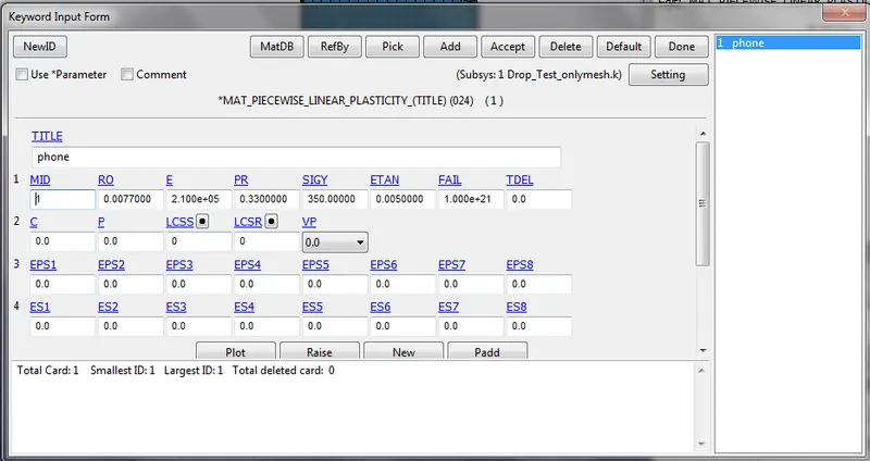
Fig.4 Material card for ground

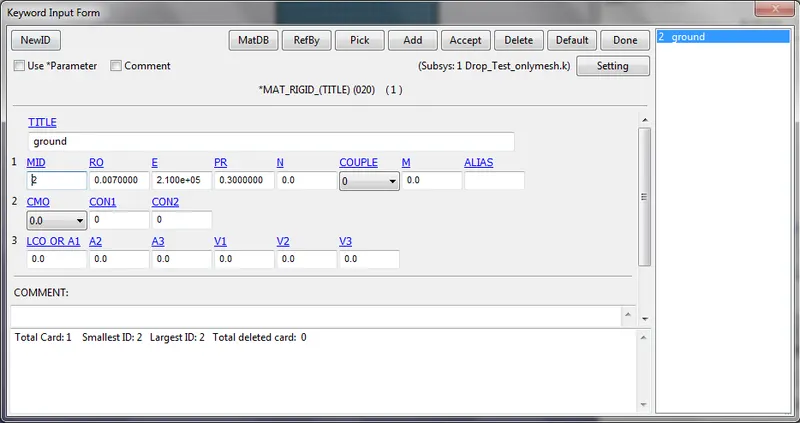
Fig. 5 Material card for ground

Create the section card for the mobile and ground

Next, we need to create the section card by giving id and thickness to the part for both ground and mobile. (as shown below)

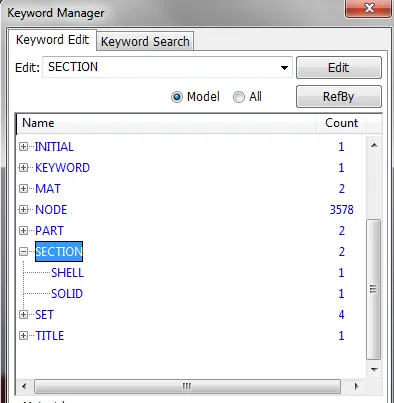
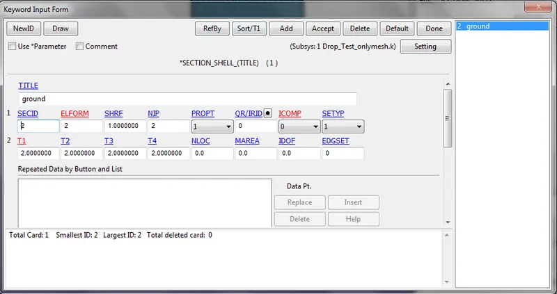
Fig.6 section card for ground

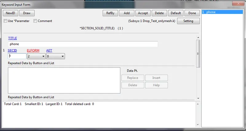
Fig.7 section card for mobile phone

Create the part card for the mobile and ground link the material card and section card to it

Set the part ID and section id with material for both the phone and ground (as shown below)

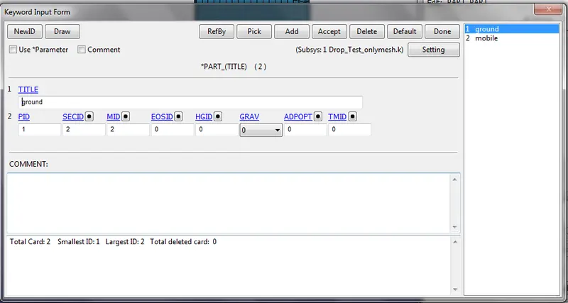
Fig. 8 Part creation for ground

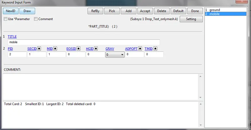
Fig. 9 Part creation for mobile

Create a contact interface between mobile and ground surface to the surface [set master and slave]

Now, we need to create the contact interface which is an automatic surface to surface.

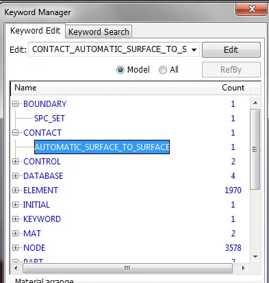
Select the master as ground and slave as mobile which is under observation where results are to be calculated. select the SSTYP and MSTYP as 3 for select by part ID

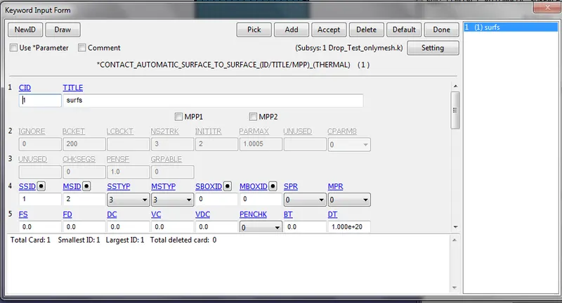
Fig. 10 Contact deployment for mobile and ground

Give the initial velocity towards the ground direction

now we need to assign an initial velocity if 10 mm/ms in negative z direction. To assign that 1st create a set part in create entity mode then give velocity card.

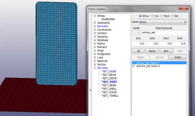
Fig. 11 part set creation

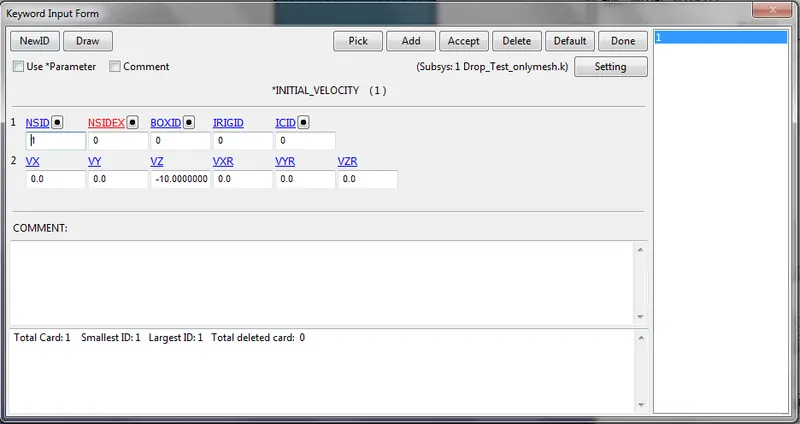
Fig. 12 Initial velocity assignment

Create the boundary condition for arresting the DOF of the plate.

Now, we need to set the boundary condition to constraint the plate motion in any DOF therefore we goto to create entity and boundary > spc (singlepoint constraint) there we need to select the peripheral node of the plate and contain them in all DOF.

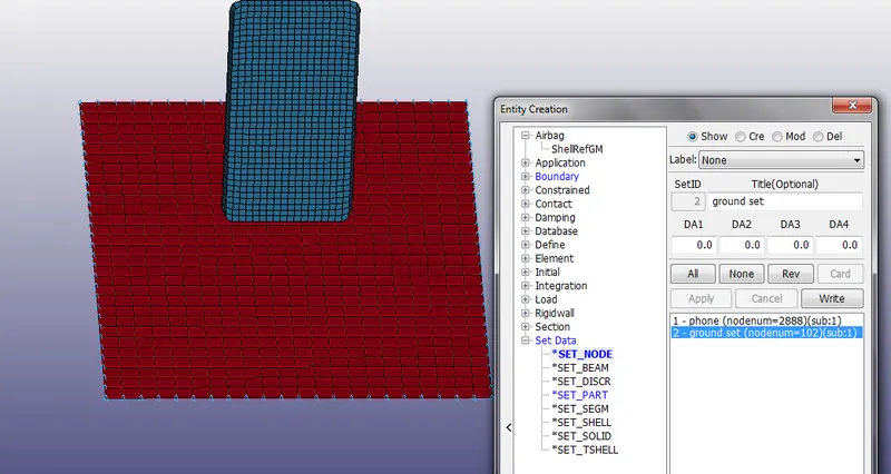
Fig. 13 Node set creation for SPC deployment

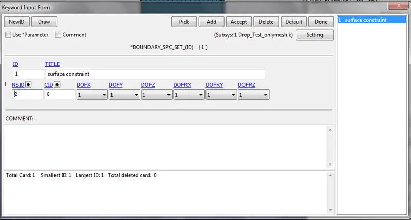
Fig. 14 Boundary SPC set up in all DOF and Node set iD(NSID) assignment as 2

Set up the termination card, control cards, and tile.

Now, we need to set up the termination, control cards, and tile card as shown below

under the database keyword we need to define the binary D3PLOT with dt as 0.1 and ASCII option and select the ELOUT, MATSUM, GLSAT... to view in the output file.

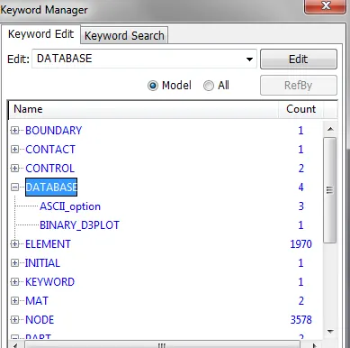
Set the DT in D3PLOT as 0.1 ms to capture the data

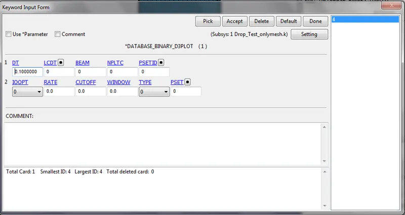
Fig.15 D3PLOT card for database with dt as 0.1 ms

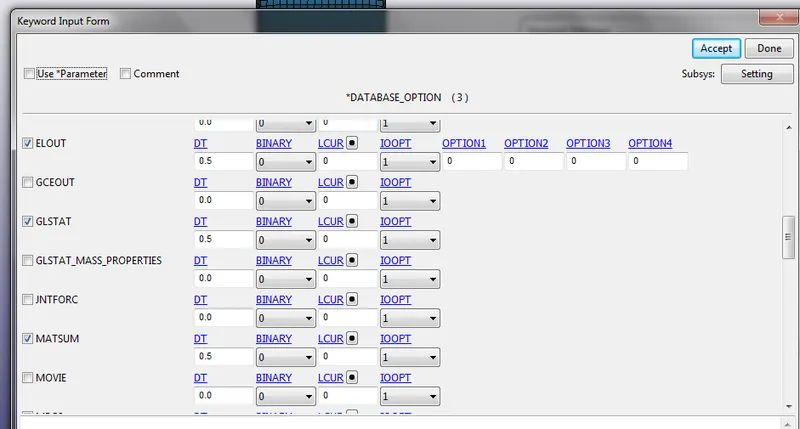
Fig.16 set the ASCII plot option

Set the termination time to 10 ms. This will include the impact as well as the rebound period for this case.

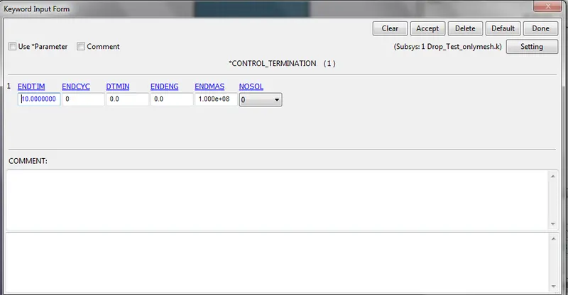
Fig. 17 Termination card setup

Run the model check and see for any errors.

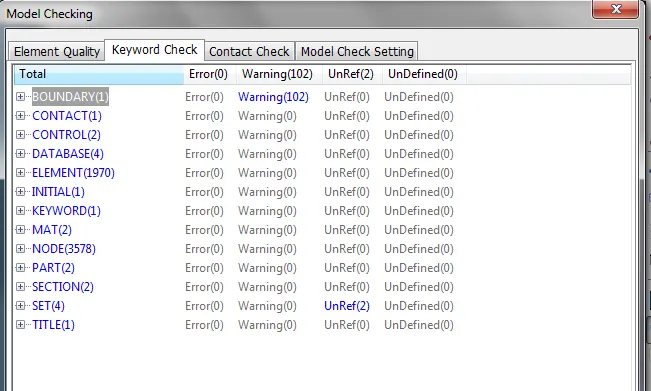
Before saving finally we need to check through the model checker to see for any error or warnings.

Run the file in the LS RUN and see the D3PLOTS (Animations+ Time History plot)

Run the file in LS RUN and then open the binary file in Ls Dyna.

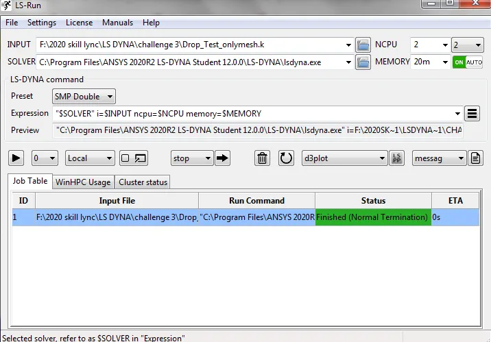
Fig.18 LS Run for solver of the .K file

Open the binary file in the ls dyna to view the animation and history plots

Open> LS Dyna binary plot > fringe component > von misses stress >Apply

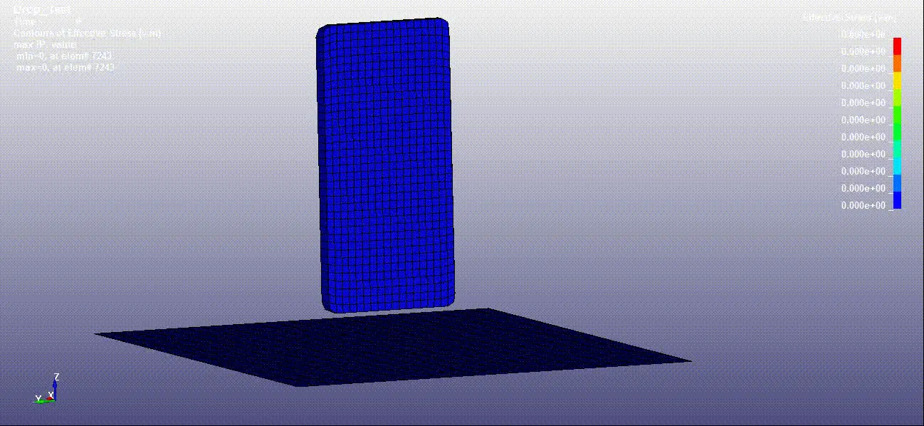
Fig. 19 Von misses stress contour animation

As we can see through the graphs for K.E and I.E vs time the k.E is at 45 E+3 units at the starting then it drops down to 15 E+3 just before 2 ms i.w when the impact happens and the at that point the K.E is converted into I.E or strain energy due to collision at the moment of impact.

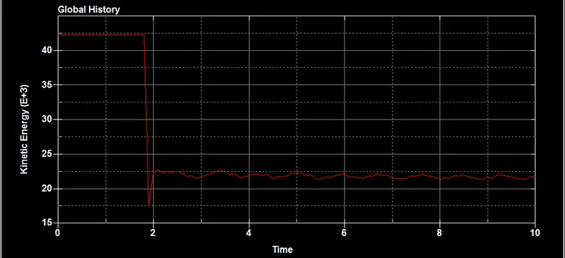
Fig. 20 K.E vs time plot (Time-History plot)

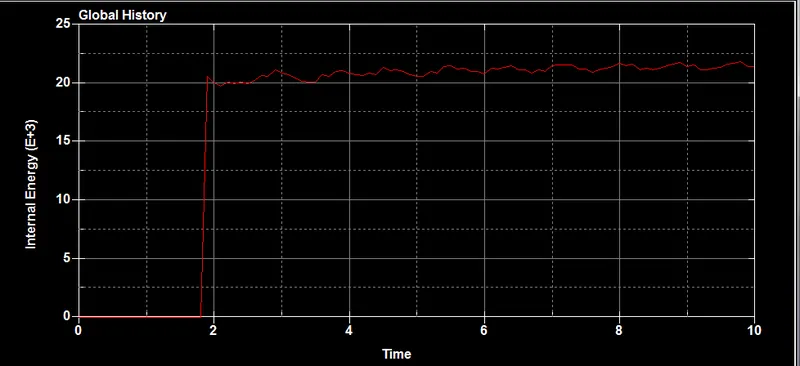
Fig. 21 I.E vs time plot (Time-History plot)

CONCLUSION:

After completing this assignment we can conclude that the procedure is very similar for setting up the solver deck file. From the run-out file, we can conclude the values of the stress and location. Also with help of time history plots, we can have the idea of how the energy is converted from one form to another.With this, we can have a clear view of the behavior of the impact between the phone and the ground.

LEARNING OUTCOME:

1. Setup of the solver deck input file
2. post processing of the output file and animation/plots capturing