Week - 3 Drop test Challenge
Simulation and Analysis of a Cell Phone Drop Test
Objective: The aim of this report is to simulate and analyze a simplified form of a vertical edge drop test of a cell phone. The pre-processing, solving, and post-processing are carried out in LS Dyna.
Geometry and Discretization: The plate is 293mm long, 220mm wide and 10 mm thick. The cell phone was modelled as a rectangular block 150.5mm long, 68.8mm wide and 5.45mm thick. The plate and phone were meshed with 1970 hexagonal elements. An additional layer of 638 quad elements was created on the surface of the plate. The phone was brought to within 5mm of the plate (in the Z-direction) using the elem tool>transform>translate option.
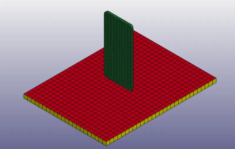
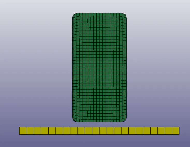
Figure 1: Isometric and front view of the drop test set up
Section Definition: Section_Shell was defined for the shell elements with ELFORM = 6 (S/R Hughes-Liu) to enable viscous hourglass control. A thickness of 2mm was given at the corner nodes 5 through-thickness integration points were defined. The rest of the car parameters were left to their default settings(see Figure 2).
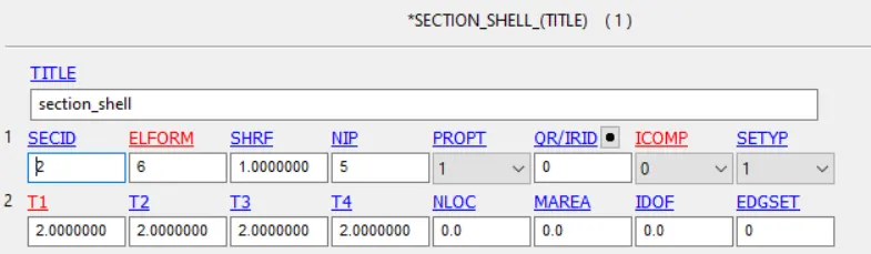
Figure 2: Shell section card
For the solid elements, Section_Solid was defined with ELFORM = 3 (fully integrated quadratic 8 node element with nodal rotations). AET was left to zero. (see Figure 3)
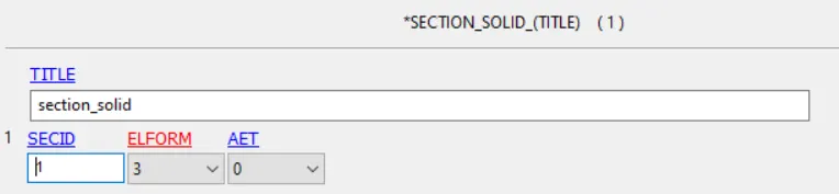
Figure 3: Solid Section Card
Hourglass Control: To prevent non-physical modes of deformation in the model, Hourglass control was introduced using Hourglass>Hourglass with a viscous type control (IHQ = 6) and an Hourglass coefficient value of 0.01. The rest of the card parameters are left to their default values.
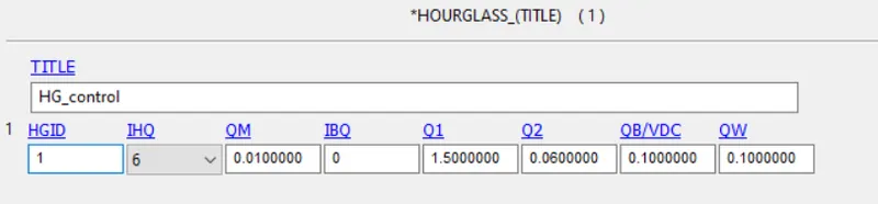
Figure 4: Hourglass Control Card
Constitutive Material Model: For the cell phone, the MAT_Piecewise_Linear_Plasticity material model was used (MAT_024). Following the kg,mm,ms unit system, the material properties were defined to simulate Polycarbonate (the material most widely used for cellphone covers these days):
| Sl No | Material Property | Magnitude | Unit |
| 1 | Density | 1.26e-06 | kg/mm3 |
| 2 | Young's Modulus | 3.24 | GPa |
| 3 | Poisson's Ratio | 0.3 | - |
| 4 | Yield Stress | 0.07 | GPa |
| 5 | Tangent Modulus | 0.65 | GPa |
| 6 | Plastic Strain to Failure | 1.0e+21 | - |
Other card parameters were left to their default values.
For the plate, MAT_Rigid was defined. This was done to simulate the rigid behavior of the plate and constrain it using the material card itself. Since the plate was defined as a rigid body, no results will be computed for this part when solving the model. The material properties of the plate (simulated as steel) were defined as follows:
| Sl No | Material Property | Magnitude | Unit |
| 1 | Density | 7.85e-06 | kg/mm3 |
| 2 | Young's Modulus | 210 | GPa |
| 3 | Poisson's Ratio |
0.3 |
- |
The rest of the parameters were left to their default values except CMO, CON1, and CON2 which were used to define the constraint (see Figure 5).
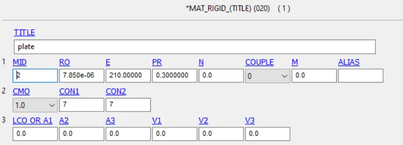
Figure 5: MAT_RIGID material card
Contact Definition: An Automatic_Surface_to_Surface interface was defined for the contact (during impact) between the cellphone and the plate. A coefficient of static friction of 0.1 was assumed. The phone was defined as the slave and the plate as the master segment. The rest of the card parameters were left to their default values.
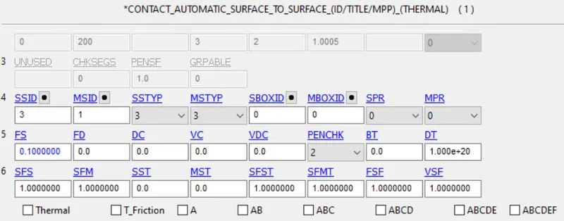
Figure 6: Surface-Surface Contact
Boundary Conditions: The plate was constrained along all its degrees of freedom using the material card itself - MAT_Rigid (see Figure 6).
The initial velocity of the phone was computed as follows:
By conservation of energy - (1/2)mv2 = mgh
=> v = `square root`(2*g*h)..................(i)
Assuming a drop height of 1.5 meters and g = 9.82e -03 mm/ms2 and substituting in equation (i), we get the initial velocity of:
v = 5.427mm/ms
This velocity is applied to all the nodes of the phone, in the negative Z-direction (global CS), using INITIAL_VELOCITY.
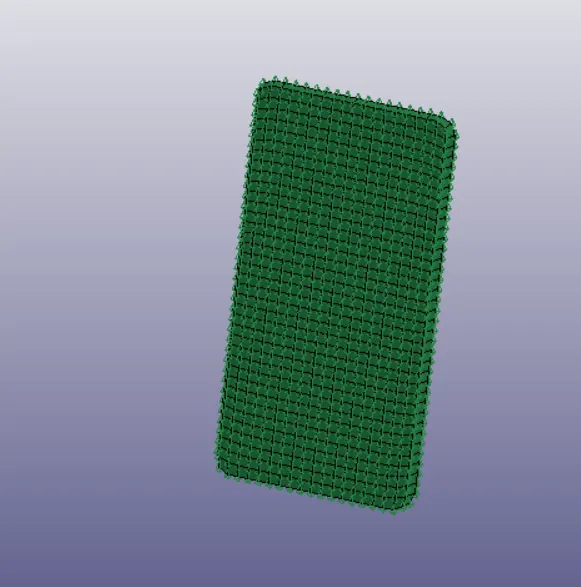
Figure 7: Initial Velocity on the Phone
Analysis Control Settings: The simulation was set to run for 2ms using CONTROL_TERMINATION. For the time step size, the Courant Friedrick Levy stability limit was computed:
`delta`t = l/c.........................(ii)
where L = characteristic element length, c = speed of sound in the element computed as:
c = `square root`(E(1-`nu`)/(`rho(1+`nu`)*(1+2`nu`))).......(iii)
The min element length in the model (before simulation) is 3.8mm. Assuming after impact, the min length becomes 2mm in certain elements and using the material properties defined in MAT_024, the stability time-step is estimated to be:
`delta`t = 0.00215 ms
Using this as a pointer, the time step for the solution is set to 0.002ms using CONTROL_TIMESTEP. The initial time step is left for auto computation and the scale factor to 0.9.
To evaluate and analyze the Hourglass Energy in the model, HGEN was set to 2 in CONTROL_ENERGY card. The same was done for sliding/contact energy.
Output Requests: For post-processing, GLSTAT, SLEOUT, RCFORC, MATSUM, and NODOUT are requested at time intervals of 0.1ms using DATABASE>ASCII option. The binary animation plot files were also requested at intervals of 0.1ms using DATABASE>BINARY_D3PLOT.
Results: The simulation terminates after a computation time of 5s. From the GLSTAT file, the time step during the run was noted to be about 1.8e-03ms which is lower than that defined in the control card. In spite of this, some amount of mass addition took place during the run (0.1% increase in mass).
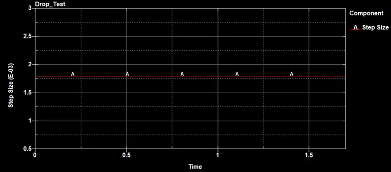
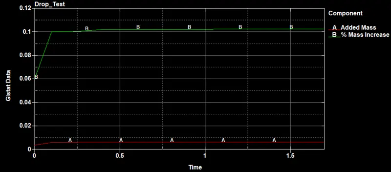
Figure 8: Time-step size Figure 9: Mass addition
The impact takes place at 0.1998ms, at which the von-mises stress in the model is the highest - 20.91MPa. The highest stress is experienced by the elements 6872 and 6059.
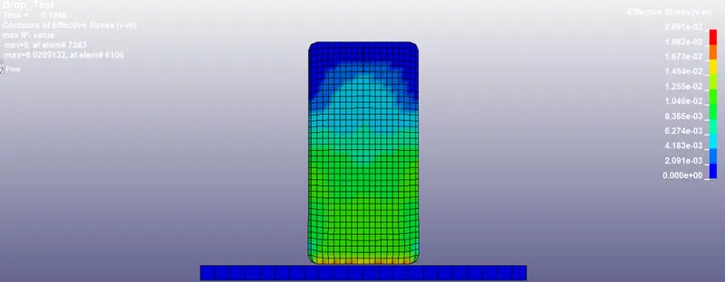
Figure 10: Von-Mises stress distribution
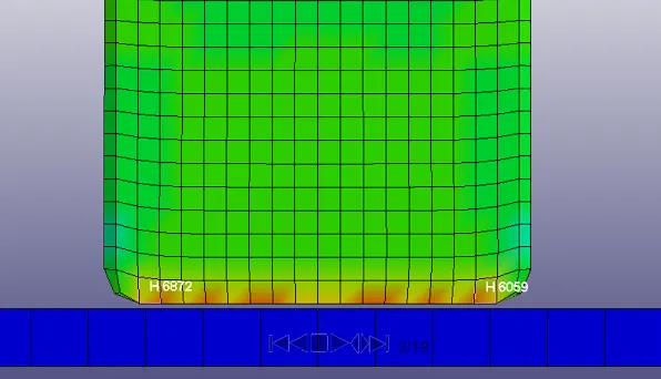
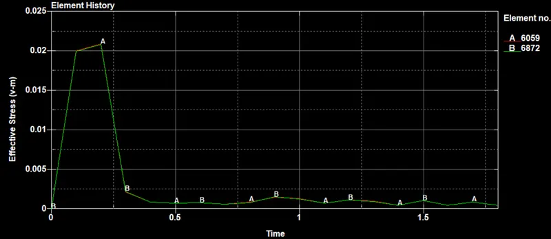
Figure 11: Von-Mises stress distribution in elements 6059 and 6872
To determine the Elastic Strain in the model, the original length of element 6872 was noted to be 4.21092mm. Using Elem Tool>Measure option, the change in length for the element was plotted.
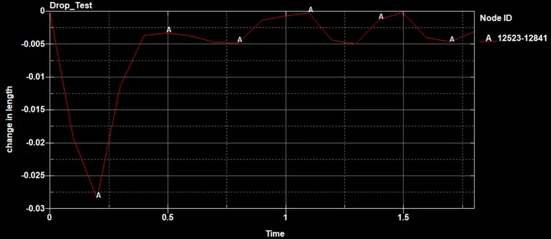
Figure 12: Change in length of element 6872
From Figure 12, it can be observed that on impact, the element compresses by 0.028mm. Therefore the elastic strain (in the Z direction) in the element is computed as:
`delta`L/L = 0.028/4.21092 = 0.006649 or 0.6649%
The kinetic energy of the model drops from 2KN-mm to about 0.6KN-mm at this point and the internal energy of the phone shoots up to about 1.3 KN-mm. A spike in the sliding or contact energy (about 0.25KN-mm) can also be seen around this time. At about 0.3ms into the run, the phone rebounds from the impact, and the energy levels almost return to their initial values (internal energy levels out at about 0.15-0.2KN-mm after rebound). The Hourglass energy in the system is zero throughout.
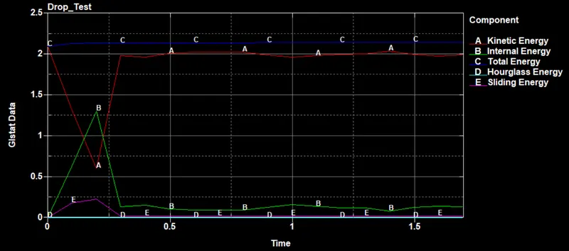
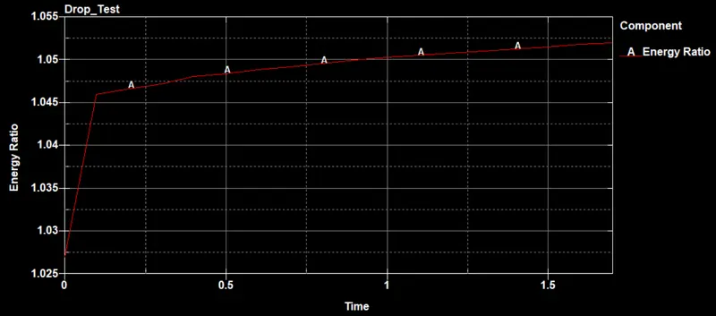
Figure 13: Energy balance Figure 14: Energy Ratio
The total energy in the system starts off at 2KN-mm but ends up being slightly more than 2KN-mm at the end of this simulation. This is also observed in the Energy Ratio plot (see Figure 14) where the said ratio peaks at a little above 1.05 (ideal value = 1.0) at the end of the simulation. This can be explained by the added mass in the system that causes this artificial increase in energy.
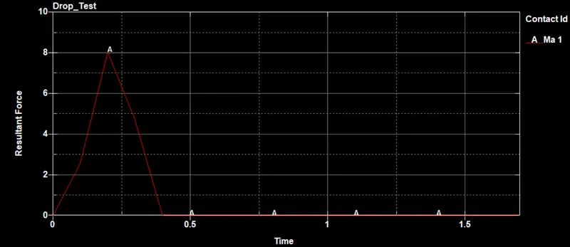
Figure 15: Interface Reaction Force
The rigid floor/plate exerts a force of 8KN on the phone on impact.
Conclusion: The max Von-Mises stress in the model is about 20MPa, which is lower than the yield stress of the material i.e. 70MPa. Therefore no plastic deformation takes place in the model and the Plastic Strain is zero. The phone retains a strain-induced energy of 0.15-0.2KN-mm as a result of the residual stress (4.48MPa). The energy conservation in the system is slightly off-balance due to the added mass which in turn was due to the time-step drop below the stability limit. With a lower time step size, this energy error can be eliminated.