Week 3 - Adiabatic Flame Temperature calculation
AIM: To write a program to analyze the effect of Equivalence ratio on adibatic flame temperature in the constant volume chamber and to compare teh results obtained using cantera
To write a program to analyze the effect of fractional heat loss on adibatic flame temperature of methane contained in the constant pressure chamber
To write a program to calculate the adiabatic flame temperature of the combustion process for a given equivalance ratio and heat loss fraction
To write a program to analyze the variation of the adiabatic flame temperature for different hydrocarbons(Alkanes, Alkenes, Alkynes)
To write a program to analyze the variation of the adiabatic flame temperature for different alkanes in a constant pressure chamber
Theory:
Adiabatic Flame Temperature(AFT):
When a combustion reaction takes place energy is released to the combustion products. If no heat is lost in this process, the temperature of the combustion products is known as the "Adiabatic Flame Temperature." The adiabatic flame temperature for a given fuel-oxidizer combination is determined by finding the final state temperature (i.e. the adiabatic flame temperature) for which the sum of the enthalpies of the reactants equal the sum of the enthalpies of the products.
The adiabatic flame temperature is the temperature of the products of a combustion reaction if no heat is lost to the external environment. By being able to calculate the adiabatic flame temperature, these fields can maximize the starting ratio of their reactions in order to get an ideal combustion result.
Case 1. Adiabatic flame temperature variation with Equivalence ratio (In constant volume-chamber) :
Python Code:
"""
General equation
CxHy + g(O2 + 3.76N2) = aCO2 + bH2O + cN2 + dO2 + eCO

x = 1; y = 4; ar = x + y/4; g = ar * (1/phi)

Stoichiometric Equation (phi = 1):

CxHy + ar(O2 + 3.76N2) = xCO2 + (y/2)H2O + 3.76(x + y/4)N2

Lean Mixture Equation

CxHy + ar(1/phi)(O2 + 3.76N2) = xCO2 + (y/2)H2O + 3.76(ar/phi)N2 + ar((1/phi)-1)O2

Rich Mixuture Equation

CxHy + ar(1/phi)(O2 + 3.76N2) = ((ar/2phi)) - x - y/2)CO2 + (y/2)H2O + 3.76(ar/phi)N2 + (2x + (y/2) - (ar/2phi))CO

"""

import matplotlib.pyplot as plt
import math

import numpy as np


R = 8.314 # J/mol*k

x = 1
y = 4

ch4_coeffs_l =  [5.14987613E+00, -1.36709788E-02, 4.91800599E-05, -4.84743026E-08, 1.66693956E-11, -1.02466476E+04, -4.64130376E+00]

o2_coeffs_l = [3.78245636E+00, -2.99673416E-03, 9.84730201E-06, -9.68129509E-09, 3.24372837E-12, -1.06394356E+03, 3.65767573E+00]

n2_coeffs_h = [0.02926640E+02, 0.14879768E-02, -0.05684760E-05, 0.10097038E-09, -0.06753351E-13, -0.09227977E+04, 0.05980528E+02]

n2_coeffs_l = [0.03298677E+02, 0.14082404E-02, -0.03963222E-04, 0.05641515E-07, -0.02444854E-10, -0.10208999E+04, 0.03950372E+02]

co2_coeffs_h = [3.85746029E+00, 4.41437026E-03, -2.21481404E-06, 5.23490188E-10, -4.72084164E-14, -4.87591660E+04, 2.27163806E+00]

h2o_coeffs_h = [3.03399249E+00, 2.17691804E-03, -1.64072518E-07, -9.70419870E-11, 1.68200992E-14, -3.00042971E+04, 4.96677010E+00]

o2_coeffs_h = [3.78245636E+00, -2.99673416E-03, 9.84730201E-06, -9.68129509E-09, 3.24372837E-12, -1.06394356E+03, 3.65767573E+00]

co_coeffs_h = [2.71518561E+00,  2.06252743E-03, -9.98825771E-07, 2.30053008E-10, -2.03647716E-14,-1.41518724E+04, 7.81868772E+00]


#Function to evaluate enthalpy

def h(T, co_effs):
	"""
	Function to evaluate enthalpy
	"""
	R = 8.314 #J/mol-k
	a1 = co_effs[0]
	a2 = co_effs[1]
	a3 = co_effs[2]
	a4 = co_effs[3]
	a5 = co_effs[4]
	a6 = co_effs[5]

	return(a1 + a2*T/2 + a3*pow(T,2)/3 + a4*pow(T,3)/4 + a5*pow(T,4)/5 + a6/T)*R*T


def f(T):
	"""
	Function that represents root finding problems
	"""
	h_co2_p = h(T,co2_coeffs_h)
	h_n2_p = h(T,n2_coeffs_h)
	h_h2o_p = h(T,h2o_coeffs_h)
	h_o2_p = h(T,o2_coeffs_h)
	h_co_p = h(T,co_coeffs_h)

	H_products = a*h_co2_p + b*h_h2o_p + c*h_n2_p + d*h_o2_p + e*h_co_p

	n_products = a + b + c + d + e
	nRT_products = n_products * R * T

	# Reactants at Standard Temperature

	Tstd=298.15
	h_ch4_r = h(Tstd,ch4_coeffs_l)
	h_o2_r = h(Tstd,o2_coeffs_l)
	h_n2_r = h(Tstd,n2_coeffs_l)

	H_reactants = h_ch4_r + g*h_o2_r + 3.76*g*h_n2_r

	n_reactants = 1 + g + 3.76*g
	nRT_reactants = n_reactants * R * T_std

	return (H_products - H_reactants) - (nRT_products - nRT_reactants)

# Functions that represents the derivative of the root finding problem
	def fprime(T):
		return (f(T+1e-6) - f(T))/1e-6


# Calculating the Temperature and storing vlaues

T_py = []
phi_min = 0.1
phi_max = 2
phi_diff = 0.1;
phi = np.arrange(phi_min, phi_max + phi_diff, phi_diff)

for i in range (0, len(phi)):

	if (phi[i] == 1):

		ar = x + y/4
		g = ar
		a = x
		b = y/2
		c = 3.76 * ar
		d = 0
		e = 0
	if (phi[i] < 1):

		ar = x + y/4
		g = ar * (1/phi[i])
		a = x
		b = y/2
		c = 3.76 * ar * (1/phi[i])
		d = ar * ((1/phi[i])-1)
		e = 0

	if (phi[i] > 1):

		ar = x + y/4
		g = ar * (1/phi[i])
		a = (2*ar/phi[i]) - x - y/2
		b = y/2
		c = 3.76 * ar * (1/phi[i])
		d = 0
		e = 2*x + y/2 - (2*ar)/phi[i]


	T_guess = 1500
	tol = 1e-6
	alpha = 0.2
	ct = 0

	while(abs(f(T_guess)) > tol):
		T_guess = T_guess - alpha * (f(T_guess) / fprime(T_guess))
		ct = ct + 1

	T_py.append(T_guess)

# Cantera Code - Exact Solution

import cantera as ct

gas = ct.Solution('gri30.xml')


T_AFT_ct = []

for i in range(0, len(phi)):

	n_total = 1 + (ar/phi[i]) + 3.76*(ar/phi[i])
	n_ch4 = 1/n_total
	n_o2 = (ar/phi[i])/n_total
	n_n2 = (3.76*(ar/phi[i]))/n_total

	gas.TPX = 298.15, 101325, {'CH4':n_ch4, 'O2':n_o2, 'N2': n_n2}
	gas.equilibrate('UV','auto')
	T_AFT_ct.append(gas.T)

	print('Equivalence Ratio = ', phi)
	print('Temperature (Python) = ', T_py)
	print('Temperature(Cantera)= ', T_AFT_ct)

# plotting the results obtained from python and Cantera


plt.plot(phi, T_py, '-o', color = 'red', label = 'Python')
plt.plot(phi, T_AFT_ct, '-o', color = 'blue', label = 'Cantera')
plt.xlabel('Equivalence Ratio', '$phi$')
plt.ylabel('Adiabatic Flame Temperature ($k$)')

plt.legend()
plt.xticks(np.arange(0, 2.1, 0.2))
plt.yticks(np.arange(400, 3000, 200))
plt.grid(which='major')
plt.minorticks_on()
plt.grid(which='minor', alpha = 0.2)
plt.show()
OUTPUT:
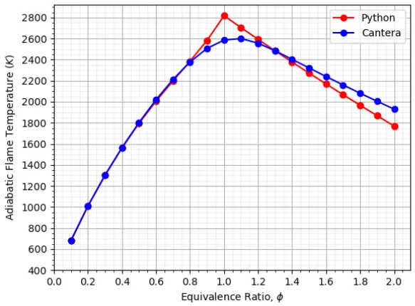
From the above graph it can be observed that at an equivalence ratio lesser than 0.8 the Adiabatic flame temperature(AFT) obtained from both python and cantera are equal. This is because the system contains enough amount of oxygen to burn the fuel in to combustion products.
2. Adiabatic flame temperature variation with Heat loss (In constant pressure-chamber) :
Python Code:
"""
General equation
CxHy + g(O2 + 3.76N2) = aCO2 + bH2O + cN2 + dO2 + eCO

x = 1; y = 4; ar = x + y/4; g = ar * (1/phi)

Stoichiometric Equation (phi = 1):

CxHy + ar(O2 + 3.76N2) = xCO2 + (y/2)H2O + 3.76(x + y/4)N2

Lean Mixture Equation

CxHy + ar(1/phi)(O2 + 3.76N2) = xCO2 + (y/2)H2O + 3.76(ar/phi)N2 + ar((1/phi)-1)O2

Rich Mixuture Equation

CxHy + ar(1/phi)(O2 + 3.76N2) = ((ar/2phi)) - x - y/2)CO2 + (y/2)H2O + 3.76(ar/phi)N2 + (2x + (y/2) - (ar/2phi))CO

"""

import matplotlib.pyplot as pyplot
import math

import numpy as np

R = 8.314 # J/mol*k

x = 1
y = 4

ch4_coeffs_l =  [5.14987613E+00, -1.36709788E-02, 4.91800599E-05, -4.84743026E-08, 1.66693956E-11, -1.02466476E+04, -4.64130376E+00]

o2_coeffs_l = [3.78245636E+00, -2.99673416E-03, 9.84730201E-06, -9.68129509E-09, 3.24372837E-12, -1.06394356E+03, 3.65767573E+00]

n2_coeffs_h = [0.02926640E+02, 0.14879768E-02, -0.05684760E-05, 0.10097038E-09, -0.06753351E-13, -0.09227977E+04, 0.05980528E+02]

n2_coeffs_l = [0.03298677E+02, 0.14082404E-02, -0.03963222E-04, 0.05641515E-07, -0.02444854E-10, -0.10208999E+04, 0.03950372E+02]

co2_coeffs_h = [3.85746029E+00, 4.41437026E-03, -2.21481404E-06, 5.23490188E-10, -4.72084164E-14, -4.87591660E+04, 2.27163806E+00]

h2o_coeffs_h = [3.03399249E+00, 2.17691804E-03, -1.64072518E-07, -9.70419870E-11, 1.68200992E-14, -3.00042971E+04, 4.96677010E+00]

o2_coeffs_h = [3.78245636E+00, -2.99673416E-03, 9.84730201E-06, -9.68129509E-09, 3.24372837E-12, -1.06394356E+03, 3.65767573E+00]

co_coeffs_h = [2.71518561E+00,  2.06252743E-03, -9.98825771E-07, 2.30053008E-10, -2.03647716E-14,-1.41518724E+04, 7.81868772E+00]

# Function to Evaluate Enthalpy

def h(T, co_effs):

	a1 = co_effs[0]
	a2 = co_effs[1]
	a3 = co_effs[2]
	a4 = co_effs[3]
	a5 = co_effs[4]
	a6 = co_effs[5]

	return(a1 + a2*T/2 + a3*pow(T,2)/3 + a4*pow(T,3)/4 + a5*pow(T,4)/5 + a6/T)*R*T

"""
	Function that represents root finding problems
	"""
def f(T, H_loss):

	# Products at Temperature T

	h_co2_p = h(T, co2_coeffs_h)
	h_n2_p = h(T, n2_coeffs_h)
	h_h2o_p = h(T, h2o_coeffs_h)
	h_o2_p = h(T, o2_coeffs_h)
	h_co_p = h(T, co_coeffs_h)

	H_products = a*h_co2_p + b*h_h2o_p + c*h_n2_p + d*h_o2_p + e*h_co_p


	# Products at Standard Temperature

	T_std = 298.15
	h_co2_p_std = h(T_std, co2_coeffs_h)
	h_n2_p_std = h(T_std, n2_coeffs_h)
	h_h2o_p_std = h(T_std, h2o_coeffs_h)
	h_o2_p_std = h(T_std, o2_coeffs_h)
	h_co_p_std = h(T_std, co_coeffs_h)

	H_products_std = a*h_co2_p_std + b*h_h2o_p_std + c*h_n2_p_std + d*h_o2_p_std + e*h_co_p_std

	# Reactants at Standard Temperature

	h_ch4_r = h(T_std, ch4_coeffs_l)
	h_o2_r = h(T_std, o2_coeffs_l)
	h_n2_r = h(T_std, n2_coeffs_l)
	H_reactants = h_ch4_r + g*h_o2_r + 3.76*g*h_n2_r

	# Lower Heating value


	LHV = H_reactants - H_products_std

	return H_products - H_reactants  + (H_loss * LHV)

# Function that represents the derivative of the root finding problem

def fprime(T):
	return (f(T+1e-6, H_loss) - f(T, H_loss)) / 1e-6

# Calculating the Temperature and Storing the values

H_loss_py = []
T_py = []
phi_py = 1
H_loss = 0
H_loss_max = 1
H_loss_diff = 0.1

if(phi_py == 1):
	ar = x +y/4
	g = ar
	a = x
	b = y/2
	c = 3.76*ar
	d = 0
	e = 0

if(phi_py < 1):
	ar = x +y/4
	g = ar * (1/phi_py)
	a = x
	b = y/2
	c = 3.76 * ar * (1/phi_py)
	d = ar * ((1/phi_py)-1)
	e = 0

if(phi_py > 1):
	ar = x +y/4
	g = ar * (1/phi_py)
	a = (2*ar/phi_py) - x - y/2
	b = y/2
	c = 3.76 * ar * (1/phi_py)
	d = 0
	e = 2*x + y/2 - (2*ar)/phi_py

T_guess = 1500
tol = 1e-6
alpha = 0.2
ct = 0

while(H_loss <= H_loss_max):

	while(abs(f(T_guess, H_loss)) > tol):
		T_guess = T_guess - alpha * (f(T_guess, H_loss) / fprime(T_guess))
		ct = ct + 1

	H_loss_py.append(H_loss)
    T_py.append(T_guess)
    H_loss = H_loss + H_loss_diff
    H_loss = round(H_loss, 1)

print('Heat Loss Fraction = ', H_loss_py)
print('Temperature = ', T_py)

# Plotting the results obtained from python


plt.plot(H_loss_py, T_py, '-o', color='red')
plt.ylim(0,2500)
plt.xticks(np.arrange(0, 1.1, 0.1))
plt.yticks(np.arrange(0, 2500, 200))
plt.xlabel('Fraction of Maximum Possible Heat Loss')
plt.ylabel('Adiabatic Flame Temperature ($k$)')
plt.grid(which='major')
plt.minorticks_on()
plt.grid(which='minor', alpha=0.2)
plt.show()
Output
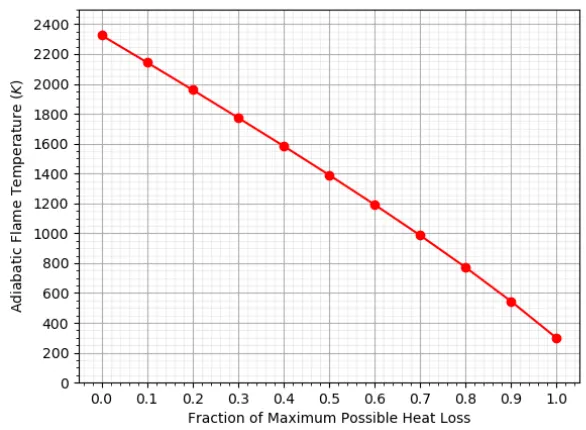
From the above graph it can be observed that as the fraction of the Maximum possible heat loss increases the Adiabatic Flame Temperature decreases.
3. Adiabatic flame temperature variation with respect to Alkane, Alkene, Alkyne :
Python Code:
"""
General equation
CxHy + g(O2 + 3.76N2) = aCO2 + bH2O + cN2 + dO2 + eCO

x = 1; y = 4; ar = x + y/4; g = ar * (1/phi)

Stoichiometric Equation (phi = 1):

CxHy + ar(O2 + 3.76N2) = xCO2 + (y/2)H2O + 3.76(x + y/4)N2

Lean Mixture Equation

CxHy + ar(1/phi)(O2 + 3.76N2) = xCO2 + (y/2)H2O + 3.76(ar/phi)N2 + ar((1/phi)-1)O2

Rich Mixuture Equation

CxHy + ar(1/phi)(O2 + 3.76N2) = ((ar/2phi)) - x - y/2)CO2 + (y/2)H2O + 3.76(ar/phi)N2 + (2x + (y/2) - (ar/2phi))CO

"""

import matplotlib.pyplot as pyplot
import math
import numpy as np

R = 8.314 # J/mol*k

x = 1
y = 4

phi_py = 1
H_loss = 0.35

ch4_coeffs_l =  [5.14987613E+00, -1.36709788E-02, 4.91800599E-05, -4.84743026E-08, 1.66693956E-11, -1.02466476E+04, -4.64130376E+00]

o2_coeffs_l = [3.78245636E+00, -2.99673416E-03, 9.84730201E-06, -9.68129509E-09, 3.24372837E-12, -1.06394356E+03, 3.65767573E+00]

n2_coeffs_h = [0.02926640E+02, 0.14879768E-02, -0.05684760E-05, 0.10097038E-09, -0.06753351E-13, -0.09227977E+04, 0.05980528E+02]

n2_coeffs_l = [0.03298677E+02, 0.14082404E-02, -0.03963222E-04, 0.05641515E-07, -0.02444854E-10, -0.10208999E+04, 0.03950372E+02]

co2_coeffs_h = [3.85746029E+00, 4.41437026E-03, -2.21481404E-06, 5.23490188E-10, -4.72084164E-14, -4.87591660E+04, 2.27163806E+00]

h2o_coeffs_h = [3.03399249E+00, 2.17691804E-03, -1.64072518E-07, -9.70419870E-11, 1.68200992E-14, -3.00042971E+04, 4.96677010E+00]

o2_coeffs_h = [3.78245636E+00, -2.99673416E-03, 9.84730201E-06, -9.68129509E-09, 3.24372837E-12, -1.06394356E+03, 3.65767573E+00]

co_coeffs_h = [2.71518561E+00,  2.06252743E-03, -9.98825771E-07, 2.30053008E-10, -2.03647716E-14,-1.41518724E+04, 7.81868772E+00]


# Function to evaluate Enthalpy

def h(T, co_effs):

	a1 = co_effs[0]
	a2 = co_effs[1]
	a3 = co_effs[2]
	a4 = co_effs[3]
	a5 = co_effs[4]
	a6 = co_effs[5]

	return(a1 + a2*T/2 + a3*pow(T,2)/3 + a4*pow(T,3)/4 + a5*pow(T,4)/5 + a6/T)*R*T


	#	Function that represents root finding problems

def f(T, H_loss):

	# Products at Temperature T

	h_co2_p = h(T, co2_coeffs_h)
	h_n2_p = h(T, n2_coeffs_h)
	h_h2o_p = h(T, h2o_coeffs_h)
	h_o2_p = h(T, o2_coeffs_h)
	h_co_p = h(T, co_coeffs_h)

	H_products = a*h_co2_p + b*h_h2o_p + c*h_n2_p + d*h_o2_p + e*h_co_p

	# Products at Standard Temperature

	T_std = 298.15
	h_co2_p_std = h(T_std, co2_coeffs_h)
	h_n2_p_std = h(T_std, n2_coeffs_h)
	h_h2o_p_std = h(T_std, h2o_coeffs_h)
	h_o2_p_std = h(T_std, o2_coeffs_h)
	h_co_p_std = h(T_std, co_coeffs_h)

	H_products_std = a*h_co2_p_std + b*h_h2o_p_std + c*h_n2_p_std + d*h_o2_p_std + e*h_co_p_std

	# Reactants at Standard Temperature

	h_ch4_r = h(T_std, ch4_coeffs_l)
	h_o2_r = h(T_std, o2_coeffs_l)
	h_n2_r = h(T_std, n2_coeffs_l)
	H_reactants = h_ch4_r + g*h_o2_r + 3.76*g*h_n2_r

	# Lower Heating value

	LHV = H_reactants - H_products_std

	return H_products - H_reactants  + (H_loss * LHV)


	# Function that represents the derivative of the root finding problem

def fprime(T):
	return (f(T+1e-6, H_loss) - f(T, H_loss)) / 1e-6

# Calculating the Temperature and Storing the values


if(phi_py == 1):
	ar = x +y/4
	g = ar
	a = x
	b = y/2
	c = 3.76*ar
	d = 0
	e = 0

if(phi_py < 1):
	ar = x +y/4
	g = ar * (1/phi_py)
	a = x
	b = y/2
	c = 3.76 * ar * (1/phi_py)
	d = ar * ((1/phi_py)-1)
	e = 0

if(phi_py > 1):
	ar = x +y/4
	g = ar * (1/phi_py)
	a = (2*ar/phi_py) - x - y/2
	b = y/2
	c = 3.76 * ar * (1/phi_py)
	d = 0
	e = 2*x + y/2 - (2*ar)/phi_py

T_guess = 1500
tol = 1e-6
alpha = 0.2
ct = 0

while(abs(f(T_guess, H_loss)) > tol):
		T_guess = T_guess - alpha * (f(T_guess, H_loss) / fprime(T_guess))
		ct = ct + 1

print('Temperature = ', T_guess)
Output:

Case 4. Adiabatic flame temperature variation with respect to a number of Carbon atom chains:
Python code:
"""
General equation
CxHy + g(O2 + 3.76N2) = aCO2 + bH2O + cN2 + dO2 + eCO

x = 1; y = 4; ar = x + y/4; g = ar * (1/phi)

Stoichiometric Equation (phi = 1):

CxHy + ar(O2 + 3.76N2) = xCO2 + (y/2)H2O + 3.76(x + y/4)N2

Lean Mixture Equation

CxHy + ar(1/phi)(O2 + 3.76N2) = xCO2 + (y/2)H2O + 3.76(ar/phi)N2 + ar((1/phi)-1)O2

Rich Mixuture Equation

CxHy + ar(1/phi)(O2 + 3.76N2) = ((ar/2phi)) - x - y/2)CO2 + (y/2)H2O + 3.76(ar/phi)N2 + (2x + (y/2) - (ar/2phi))CO

"""
import matplotlib.pyplot as plt
import math
import numpy as np

R = 8.314 # J/mol*k

x = 2
y = 6
carbon_type = 1

c2h6_coeffs_l = [4.29142492E+00, -5.50154270E-03, 5.99438288E-05, -7.08466285E-08, 2.68685771E-11, -1.15222055E+04, 2.66682316E+00]

c2h4_coeffs_l = [3.95920148E+00, -7.57052247E-03, 5.70990292E-05, -6.91588753E-08, 2.69884373E-11,  5.08977593E+03, 4.09733096E+00]

c2h2_coeffs_l = [8.08681094E-01,  2.33615629E-02, -3.55171815E-05, 2.80152437E-08, -8.50072974E-12, 2.64289807E+04, 1.39397051E+01]

o2_coeffs_l = [3.78245636E+00, -2.99673416E-03, 9.84730201E-06, -9.68129509E-09, 3.24372837E-12, -1.06394356E+03, 3.65767573E+00]

n2_coeffs_h = [0.02926640E+02, 0.14879768E-02, -0.05684760E-05, 0.10097038E-09, -0.06753351E-13, -0.09227977E+04, 0.05980528E+02]

n2_coeffs_l = [0.03298677E+02, 0.14082404E-02, -0.03963222E-04, 0.05641515E-07, -0.02444854E-10, -0.10208999E+04, 0.03950372E+02]

co2_coeffs_h = [3.85746029E+00, 4.41437026E-03, -2.21481404E-06, 5.23490188E-10, -4.72084164E-14, -4.87591660E+04, 2.27163806E+00]

h2o_coeffs_h = [3.03399249E+00, 2.17691804E-03, -1.64072518E-07, -9.70419870E-11, 1.68200992E-14, -3.00042971E+04, 4.96677010E+00]

o2_coeffs_h = [3.78245636E+00, -2.99673416E-03, 9.84730201E-06, -9.68129509E-09, 3.24372837E-12, -1.06394356E+03, 3.65767573E+00]

co_coeffs_h = [2.71518561E+00,  2.06252743E-03, -9.98825771E-07, 2.30053008E-10, -2.03647716E-14,-1.41518724E+04, 7.81868772E+00]

# Function to evaluate Enthalpy

def h(T, co_effs):

	R = 8.314 #J/mol-K
	a1 = co_effs[0]
	a2 = co_effs[1]
	a3 = co_effs[2]
	a4 = co_effs[3]
	a5 = co_effs[4]
	a6 = co_effs[5]

return(a1 + a2*T/2 + a3*pow(T,2)/3 + a4*pow(T,3)/4 + a5*pow(T,4)/5 + a6/T)*R*T


	#Function that represents root finding problems

def f(T, H_loss):

	# Products at Temperature T

	h_co2_p = h(T, co2_coeffs_h)
	h_n2_p = h(T, n2_coeffs_h)
	h_h2o_p = h(T, h2o_coeffs_h)
	h_o2_p = h(T, o2_coeffs_h)
	h_co_p = h(T, co_coeffs_h)
	H_products = a*h_co2_p + b*h_h2o_p + c*h_n2_p + d*h_o2_p + e*h_co_p

	# Products at Standard Temperature

	T_std = 298.15
	h_co2_p_std = h(T_std, co2_coeffs_h)
	h_n2_p_std = h(T_std, n2_coeffs_h)
	h_h2o_p_std = h(T_std, h2o_coeffs_h)
	h_o2_p_std = h(T_std, o2_coeffs_h)
	h_co_p_std = h(T_std, co_coeffs_h)

	H_products_std = a*h_co2_p_std + b*h_h2o_p_std + c*h_n2_p_std + d*h_o2_p_std + e*h_co_p_std

	# Reactants at Standard Temperature

	if carbon_type == 1:
		h_hydrocarbon_r = h(T_std, c2h6_coeffs_l)

	elif carbon_type == 2:
	    h_hydrocarbon_r = h(T_std, c2h4_coeffs_l)

	elif carbon_type == 3:
		h_hydrocarbon_r = h(T_std, c2h2_coeffs_l)

	h_o2_r = h(T_std, o2_coeffs_l)
	h_n2_r = h(T_std, n2_coeffs_l)
	H_reactants = h_hydrocarbon_r + g*h_o2_r + 3.76*g*h_n2_r

	# Lower Heating value

	LHV = H_reactants - H_products_std

	return H_products - H_reactants  + (H_loss * LHV)

# Function that represents the derivative of the root finding problem

def fprime(T):
	return (f(T+1e-6, H_loss) - f(T, H_loss)) / 1e-6

# Calculating the Temperature and storing the values

T_py = []

for carbon_type in range (1,4):

	phi_py = 1
	H_loss = 0.35


	if carbon_type == 1:
		x = 2
		y = 6
	elif carbon_type == 2:
		x = 2
		y = 4
	elif carbon_type == 3:
		x = 2
		y = 2

if(phi_py == 1):
	ar = x +y/4
	g = ar
	a = x
	b = y/2
	c = 3.76*ar
	d = 0
	e = 0

if(phi_py < 1):
	ar = x +y/4
	g = ar * (1/phi_py)
	a = x
	b = y/2
	c = 3.76 * ar * (1/phi_py)
	d = ar * ((1/phi_py)-1)
	e = 0

if(phi_py > 1):
	ar = x +y/4
	g = ar * (1/phi_py)
	a = (2*ar/phi_py) - x - y/2
	b = y/2
	c = 3.76 * ar * (1/phi_py)
	d = 0
	e = 2*x + y/2 - (2*ar)/phi_py

T_guess = 1500
tol = 1e-6
alpha = 0.2
ct = 0

while(abs(f(T_guess, H_loss)) > tol):
		T_guess = T_guess - alpha * (f(T_guess, H_loss) / fprime(T_guess))
		ct = ct + 1

print('Temperature (Python) = ', T_py)

# Plotting results obtained from Python

x_bar = ['Ethane','Ethene','Ethyne']
x_pos = [i for i, _ in enumerate(x_bar)]

fig, ax = plt.subplots()
rects1 = ax.bar(x_pos, T_py)
plt.ylim(1700,2100)


plt.xlabel("Types of Hydrocarbon")
plt.ylabel("Adiabatic Flame Temperature ($K$)")

plt.xticks(x_pos, x_bar)
plt.minorticks_on()

plt.grid(which = 'major', linestyle='-',linewidth='0.2')
plt.grid(which = 'minor', linestyle=':',linewidth='0.2')


def autolabel(rects):

	for rect in rects:
		height = rect.get_height()
		ax.text(rect.get_x() + rect.get_width()/2., height, '%0.3f K', % float(height), ha = 'center', va = 'bottom')
autolabel(rects1)

plt.show()
Output
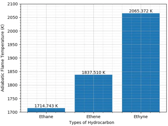
Alkynes has more number of bonds compared to alkanes and alkenes. From the above graph we can observe that the Aidabatic Flame Temperature(AFT) increases as the number of bonds increases.
Case 5: Adiabatic Flame Temperature variation for different alkanes
Python Code:
"""
General equation
CxHy + g(O2 + 3.76N2) = aCO2 + bH2O + cN2 + dO2 + eCO

x = 1; y = 4; ar = x + y/4; g = ar * (1/phi)

Stoichiometric Equation (phi = 1):

CxHy + ar(O2 + 3.76N2) = xCO2 + (y/2)H2O + 3.76(x + y/4)N2

Lean Mixture Equation

CxHy + ar(1/phi)(O2 + 3.76N2) = xCO2 + (y/2)H2O + 3.76(ar/phi)N2 + ar((1/phi)-1)O2

Rich Mixuture Equation

CxHy + ar(1/phi)(O2 + 3.76N2) = ((ar/2phi)) - x - y/2)CO2 + (y/2)H2O + 3.76(ar/phi)N2 + (2x + (y/2) - (ar/2phi))CO

"""
import matplotlib.pyplot as plt
import math
import numpy as np

R = 8.314 # J/mol*k

x = 2
y = 6
carbon_type = 1

c2h6_coeffs_l = [4.29142492E+00, -5.50154270E-03, 5.99438288E-05, -7.08466285E-08, 2.68685771E-11, -1.15222055E+04, 2.66682316E+00]

ch4_coeffs_l =  [5.14987613E+00, -1.36709788E-02, 4.91800599E-05, -4.84743026E-08, 1.66693956E-11, -1.02466476E+04, -4.64130376E+00]

c3h8_coeffs_1 = [0.93355381E+00,  0.26424579E-01, 0.61059727E-05, -0.21977499E-07, 0.95149253E-11, -0.13958520E+05, 0.19201691E+02]

o2_coeffs_l = [3.78245636E+00, -2.99673416E-03, 9.84730201E-06, -9.68129509E-09, 3.24372837E-12, -1.06394356E+03, 3.65767573E+00]

n2_coeffs_h = [0.02926640E+02, 0.14879768E-02, -0.05684760E-05, 0.10097038E-09, -0.06753351E-13, -0.09227977E+04, 0.05980528E+02]

n2_coeffs_l = [0.03298677E+02, 0.14082404E-02, -0.03963222E-04, 0.05641515E-07, -0.02444854E-10, -0.10208999E+04, 0.03950372E+02]

co2_coeffs_h = [3.85746029E+00, 4.41437026E-03, -2.21481404E-06, 5.23490188E-10, -4.72084164E-14, -4.87591660E+04, 2.27163806E+00]

h2o_coeffs_h = [3.03399249E+00, 2.17691804E-03, -1.64072518E-07, -9.70419870E-11, 1.68200992E-14, -3.00042971E+04, 4.96677010E+00]

o2_coeffs_h = [3.78245636E+00, -2.99673416E-03, 9.84730201E-06, -9.68129509E-09, 3.24372837E-12, -1.06394356E+03, 3.65767573E+00]

co_coeffs_h = [2.71518561E+00,  2.06252743E-03, -9.98825771E-07, 2.30053008E-10, -2.03647716E-14,-1.41518724E+04, 7.81868772E+00]

# Function to evaluate Enthalpy

def h(T, co_effs):


	R = 8.314 #J/mol-K
	a1 = co_effs[0]
	a2 = co_effs[1]
	a3 = co_effs[2]
	a4 = co_effs[3]
	a5 = co_effs[4]
	a6 = co_effs[5]

return(a1 + a2*T/2 + a3*pow(T,2)/3 + a4*pow(T,3)/4 + a5*pow(T,4)/5 + a6/T)*R*T


	#	Function that represents root finding problems

def f(T, H_loss):

	# Products at Temperature T

	h_co2_p = h(T, co2_coeffs_h)
	h_n2_p = h(T, n2_coeffs_h)
	h_h2o_p = h(T, h2o_coeffs_h)
	h_o2_p = h(T, o2_coeffs_h)
	h_co_p = h(T, co_coeffs_h)
	H_products = a*h_co2_p + b*h_h2o_p + c*h_n2_p + d*h_o2_p + e*h_co_p

	# Products at Standard Temperature

	T_std = 298.15
	h_co2_p_std = h(T_std, co2_coeffs_h)
	h_n2_p_std = h(T_std, n2_coeffs_h)
	h_h2o_p_std = h(T_std, h2o_coeffs_h)
	h_o2_p_std = h(T_std, o2_coeffs_h)
	h_co_p_std = h(T_std, co_coeffs_h)

	H_products_std = a*h_co2_p_std + b*h_h2o_p_std + c*h_n2_p_std + d*h_o2_p_std + e*h_co_p_std

	# Reactants at Standard Temperature

	if carbon_type == 1:
		h_hydrocarbon_r = h(T_std, ch4_coeffs_l)

	elif carbon_type == 2:
	    h_hydrocarbon_r = h(T_std, c2h6_coeffs_l)

	elif carbon_type == 3:
		h_hydrocarbon_r = h(T_std, c3h8_coeffs_l)

	h_o2_r = h(T_std, o2_coeffs_l)
	h_n2_r = h(T_std, n2_coeffs_l)
	H_reactants = h_hydrocarbon_r + g*h_o2_r + 3.76*g*h_n2_r

	# Lower Heating value

	LHV = H_reactants - H_products_std

	return H_products - H_reactants  + (H_loss * LHV)

# Function that represents the derivative of the root finding problem

def fprime(T):
	return (f(T+1e-6, H_loss) - f(T, H_loss)) / 1e-6

# Calculating the Temperature and storing the values

T_py = []

for carbon_type in range (1,4):

	phi_py = 1
	H_loss = 0


	if carbon_type == 1:
		x = 1
		y = 4
	elif carbon_type == 2:
		x = 2
		y = 6
	elif carbon_type == 3:
		x = 3
		y = 8

if(phi_py == 1):
	ar = x +y/4
	g = ar
	a = x
	b = y/2
	c = 3.76*ar
	d = 0
	e = 0

if(phi_py < 1):
	ar = x +y/4
	g = ar * (1/phi_py)
	a = x
	b = y/2
	c = 3.76 * ar * (1/phi_py)
	d = ar * ((1/phi_py)-1)
	e = 0

if(phi_py > 1):
	ar = x +y/4
	g = ar * (1/phi_py)
	a = (2*ar/phi_py) - x - y/2
	b = y/2
	c = 3.76 * ar * (1/phi_py)
	d = 0
	e = 2*x + y/2 - (2*ar)/phi_py

T_guess = 1500
tol = 1e-6
alpha = 0.2
ct = 0

while(abs(f(T_guess, H_loss)) > tol):
		T_guess = T_guess - alpha * (f(T_guess, H_loss) / fprime(T_guess))
		ct = ct + 1

T_py.append(T_guess)

print('Temperature (Python) = ', T_py)

# Plotting results obtained from Python

x_bar = ['Methane','Ethane','Propane']
x_pos = [i for i, _ in enumerate(x_bar)]

fig, ax = plt.subplots()
rects1 = ax.bar(x_pos, T_py)
plt.ylim(2300,2400)

plt.xlabel("Types of Alkane")
plt.ylabel("Adiabatic Flame Temperature ($K$)")

plt.xticks(x_pos, x_bar)
plt.minorticks_on()

plt.grid(which = 'major', linestyle='-',linewidth='0.2')
plt.grid(which = 'minor', linestyle=':',linewidth='0.2')

def autolabel(rects):

	for rect in rects:
		height = rect.get_height()
		ax.text(rect.get_x() + rect.get_width()/2., height, '%0.3f K', % float(height), ha = 'center', va = 'bottom')
autolabel(rects1)

plt.show()
Output:
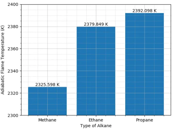
From the above graph it can be observed that as the number of carbon atoms in the Alkane increases the Adiabatic Flame Temperature(AFT) of the respective alkane increases