Week 3 - Adiabatic Flame Temperature calculation
ADIABATIC FLAME TEMPERATURE CALCULATION USING PYTHON AND CANTERA
OBJECTIVE : To find the adiabatic flame temperature of the various fuels using python and validate the results using cantera.
INTRODUCTION
Adiabatic flame temperature (AFT): The temperature of the combustion products when no heat is lost to the surroundings in this process, is known as the Adiabatic Flame Temperature. There are two process on which AFT depends, they are 1. Constant volume and 2. constant pressure. AFT is considered as maximum temperature that a fuel can generate during the combustion process. So, AFT becomes crucial data to determine the materials that can withstand the high temperatures used in developing the combustion engine.
In this challenge, we will consider both cases Constant volume and constant pressure to determine the AFT as well as experiment with the fuels to demonstrate dependence of the AFT on them. All the results in each case will be compared to the Cantera results. Cantera results are more accurate because if minimizes the Gibbs free energy to maintain equilibrium. In cantera. we used constant internal energy and specific volume to equilibrate the solution
To determine the AFT of the fuels, we need to know the enthalpies of the species involved in the reaction process. Thermo data of the species are taken from NASA POLYNOMIALS. Once the total enthalpy of the reaction is derived then Newton-Raphson technique which is a iterative method is used to find the root of the function. Once the root of the function satisfies the tolerance value then root value is consider as the AFT of the particular fuel.
CASE-I: Effect of equivalence ratio of methane fuel on AFT using Constant volume process.
'''
program for calculating the adiabatic flame temperature of the methane fuel for variours equivalence ratios at constant volume

Equvialence ratio is defined as the ratio of the actual fuel/air ratio to the stoichiometric fuel/air ratio. It is denoted by 'phi'.

phi = The actual(fuel/air ratio)/stochiometric(fuel/air ratio)

Stochiometric reaction: Stoichiometric combustion occurs when all the oxygen is consumed in the reaction, and there is no molecular oxygen(O2) in the products.

If the equivalence ratio is equal to one, the combustion is stoichiometric. phi = 1

CH4 + 2(O2 + 3.76N2) = CO2 + 2H20 + 7.52n2

If phi < 1, the combustion is lean with excess air which contains an extra oxygen on the product side.

CH4 + x(O2 + 3.76N2) = aCO2 + bH20 + 7.52N2 + c*O2

calculating the coefficients. a = 1, b = 2.

equivalence ratio = phi,
no of moles fuel = 1,
no of moles of air = x,

phi = (1/x)/1/2 => x = 2/phi

c = 2/phi-2

then above equation will be

CH4 + 2/phi(O2 + 3.76N2) = CO2 + 2H20 + 7.52/phi*N2 + (2/phi-2)*O2

If >1, the combustion is rich with incomplete combustion and forms carbon monoxide on the product side.

CH4 + x(O2 + 3.76N2) = aCO2 + bH20 + 7.52/phi*N2 + d*CO

deriveing the coefficients

a = 4/phi-3
b = 2
d = 4-4/phi

CH4 + 2/phi(O2 + 3.76N2) = (4/phi-3)CO2 + 2H20 + 7.52/phi*N2 + (4-4/phi)CO

'''
import matplotlib.pyplot as plt
import math
import cantera as ct
import numpy as np

R = 8.314 #j/mol-k
Tstd = 298.15

def h(T,co_effs):

	# function for evaluating enthalpy
	R = 8.314 #j/mol-k
	a1 = co_effs[0]
	a2 = co_effs[1]
	a3 = co_effs[2]
	a4 = co_effs[3]
	a5 = co_effs[4]
	a6 = co_effs[5]

	return (a1 + a2*T/2 + a3*pow(T,2)/3 +  a4*pow(T,3)/4 +  a5*pow(T,4)/5 + a6/T)*R*T

# Thermodata of the reactants at T<1000
ch4_coeff_l = [5.14987613E+00,-1.36709788E-02,4.91800599E-05,-4.84743026E-08,1.66693956E-11,-1.02466476E+04,-4.64130376E+00]
o2_coeff_l = [3.78245636E+00,-2.99673416E-03,9.84730201E-06,-9.68129509E-09,3.24372837E-12,-1.06394356E+03,3.65767573E+00]
n2_coeff_l = [0.03298677E+02,0.14082404E-02,-0.03963222E-04,0.05641515E-07,-0.02444854E-10,-0.10208999E+04,0.03950372E+02]

# Thermodata of the products at T>1000
n2_coeff_h = [0.02926640E+02,0.14879768E-02,-0.05684760E-05,0.10097038E-09,-0.06753351E-13,-0.09227977E+04,0.05980528E+02]
co2_coeff_h = [3.85746029E+00,4.41437026E-03,-2.21481404E-06,5.23490188E-10,-4.72084164E-14,-4.87591660E+04,2.27163806E+00]
h20_coeff_h = [3.03399249E+00,2.17691804E-03,-1.64072518E-07,-9.70419870E-11,1.68200992E-14,-3.00042971E+04,4.96677010E+00]
co_coeff_h = [2.71518561E+00,2.06252743E-03,-9.98825771E-07,2.30053008E-10,-2.03647716E-14,-1.41518724E+04,7.81868772E+00]
o2_coeff_h = [3.28253784E+00,1.48308754E-03,-7.57966669E-07,2.09470555E-10,-2.16717794E-14,-1.08845772E+03,5.45323129E+00]

def f(T,phi):

	h_ch4_r = h(Tstd,ch4_coeff_l)
	h_o2_r = h(Tstd,o2_coeff_l)
	h_n2_r = h(Tstd,n2_coeff_l)

	H_reactants = h_ch4_r + (2/phi)*h_o2_r + (7.52/phi)*h_n2_r
	N_reactants = (1 + 2/phi + (7.52/phi))*R*Tstd

	h_co2_p = h(T,co2_coeff_h)
	h_h20_p = h(T,h20_coeff_h)
	h_n2_p = h(T,n2_coeff_h)
	h_o2_p = h(T,o2_coeff_h)
	h_co_p = h(T,co_coeff_h)

	if phi >= 1:
		H_products = (4/phi-3)*h_co2_p + 2*h_h20_p + 7.52/phi*h_n2_p + (4-4/phi)*h_co_p
		N_products = ((4/phi-3) + 2 + (7.52/phi) + (4-4/phi))*R*T
	elif phi < 1:
		H_products = h_co2_p + 2*h_h20_p + 7.52/phi*h_n2_p + (2/phi-2)*h_o2_p
		N_products = (1 + 2 + 7.52/phi + (2/phi-2))*R*T

	return (H_products - H_reactants) - (N_products - N_reactants)

def fprime(T,phi):
	return (f(T+1e-6,phi) - f(T,phi))/(1e-6)

'''
performing newton-rhapson iteration

'''

alpha = 0.2
tol = 1e-3
phi = np.linspace(0.1,2,25)
AFT_py = []

for i in range(0,len(phi)):
	T_guess = 1500
	while abs(f(T_guess,phi[i])) > tol:
		T_guess = T_guess - alpha*(f(T_guess,phi[i])/fprime(T_guess,phi[i]))
	AFT_py.append(T_guess)
print(AFT_py)

# Adiabatic flame temperature obtained by using Cantera library.

gas = ct.Solution('gri30.xml')
AFT_ct = []
for i in range(0,len(phi)):
	N_tot = 1 + 2/phi[i] + 7.52/phi[i]
	N_ch4 = 1/N_tot
	N_o2 = (2/phi[i])/N_tot
	N_n2 = (7.52/phi[i])/N_tot

	# fuel-air properties
	gas.TPX = 298.15, 101325,{'CH4':N_ch4,'O2':N_o2,'N2':N_n2}
	gas.equilibrate('UV','auto') # U = internal energy, V = Specific volume, auto = solver selection
	AFT_ct.append(gas.T)
print(AFT_ct)

plt.plot(phi,AFT_py,'-*',color='blue',label='Python')
plt.plot(phi,AFT_ct,'-*',color='red',label='Cantera')
plt.xlabel('Equivalence Ratio (phi)')
plt.ylabel('Adiabatic flame temperature (K)')
plt.grid('on')
plt.legend(fontsize = 12)
plt.title('Equivalence ratio vs AFT of Methane-Air combustion')
plt.show()
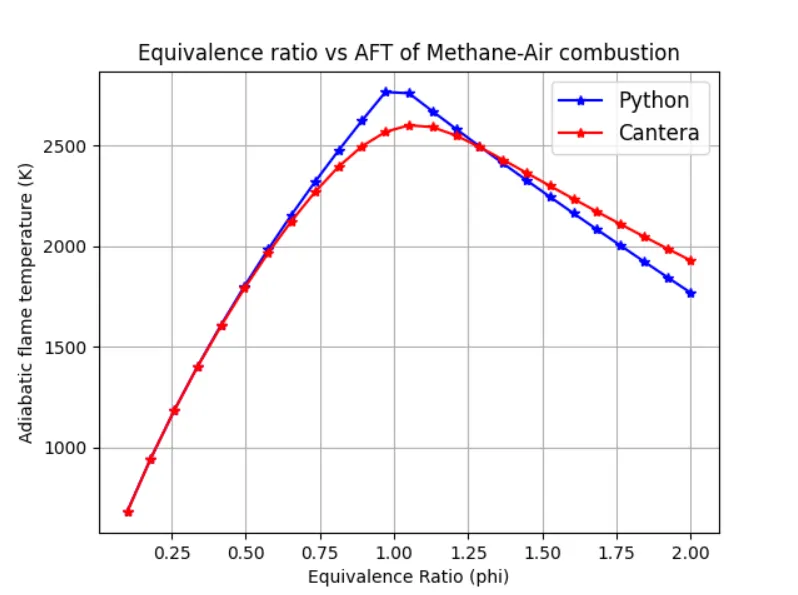
From the above graph we can observe that when the equivalence ratio around 1 there is the highest difference between the curves. In the python, we have used ideal case which is stochiometric reaction so there are very less spices to calculate the complete AFT, In case of Cantera, It has consider more species. However, differences between the curves at each point is less.
CASE-2 : Flame temperature of the methane fuel is calculated using constant pressure process with heat loss = 0.35.
LHV = Lower heating value determines the total amount of heat that can be generated from combustion of unit fuel. It is calculated by substracting the enthalpies of the reactants and products at standard temperature of 298.15(k).
In this case combustion is stoichiometric. If Heat loss (H_loss) = 1, then heat is completely lost to the surroundings, If H_loss = 0, then heat remained within the system which gives maximum temperature possible in combustion that is AFT.
'''
program for calculating the adiabatic flame temperature of the methane fuel with heat loss = 0.35in the products.

If the equivalence ratio is equal to one, the combustion is stoichiometric. phi = 1

CH4 + 2O2 + 7.52N2 = CO2 + 2H20 + 7.52N2

'''
import matplotlib.pyplot as plt
import numpy as np

R = 8.314 #j/mol-k
Tstd = 298.15

def h(T,co_effs):

	# function for evaluating enthalpy
	R = 8.314 #j/mol-k
	a1 = co_effs[0]
	a2 = co_effs[1]
	a3 = co_effs[2]
	a4 = co_effs[3]
	a5 = co_effs[4]
	a6 = co_effs[5]

	return (a1 + a2*T/2 + a3*pow(T,2)/3 +  a4*pow(T,3)/4 +  a5*pow(T,4)/5 + a6/T)*R*T

# Thermodata of the reactants at T<1000
ch4_coeff_l = [5.14987613E+00,-1.36709788E-02,4.91800599E-05,-4.84743026E-08,1.66693956E-11,-1.02466476E+04,-4.64130376E+00]
o2_coeff_l = [3.78245636E+00,-2.99673416E-03,9.84730201E-06,-9.68129509E-09,3.24372837E-12,-1.06394356E+03,3.65767573E+00]
n2_coeff_l = [0.03298677E+02,0.14082404E-02,-0.03963222E-04,0.05641515E-07,-0.02444854E-10,-0.10208999E+04,0.03950372E+02]

# Thermodata of the products at T>1000
n2_coeff_h = [0.02926640E+02,0.14879768E-02,-0.05684760E-05,0.10097038E-09,-0.06753351E-13,-0.09227977E+04,0.05980528E+02]
co2_coeff_h = [3.85746029E+00,4.41437026E-03,-2.21481404E-06,5.23490188E-10,-4.72084164E-14,-4.87591660E+04,2.27163806E+00]
h20_coeff_h = [3.03399249E+00,2.17691804E-03,-1.64072518E-07,-9.70419870E-11,1.68200992E-14,-3.00042971E+04,4.96677010E+00]

#maximum heat loss possible. LHV = Lower heating value
LHV = h(Tstd,ch4_coeff_l)+2*h(Tstd,o2_coeff_l)+7.52*h(Tstd,n2_coeff_l)-h(Tstd,co2_coeff_h)-2*h(Tstd,h20_coeff_h)-7.52*h(Tstd,n2_coeff_h)


def f(T,H_loss):

	h_ch4_r = h(Tstd,ch4_coeff_l)
	h_o2_r = h(Tstd,o2_coeff_l)
	h_n2_r = h(Tstd,n2_coeff_l)

	H_reactants = h_ch4_r + 2*h_o2_r + 7.52*h_n2_r

	h_co2_p = h(T,co2_coeff_h)
	h_h20_p = h(T,h20_coeff_h)
	h_n2_p = h(T,n2_coeff_h)

	H_products = h_co2_p + 2*h_h20_p + 7.52*h_n2_p

	Loss = H_loss*LHV

	return H_products - H_reactants + Loss

def fprime(T,H_loss):
	return (f(T+1e-6,H_loss) - f(T,H_loss))/(1e-6)

'''
performing newton-rhapson iteration

'''
T_guess = 1500
alpha = 0.2
tol = 1e-3
H_loss = np.linspace(0.05,1,20)
AFT_cp = []

for i in range(0,len(H_loss)):
	while abs(f(T_guess,H_loss[i])) > tol:
		T_guess = T_guess - alpha*(f(T_guess,H_loss[i])/fprime(T_guess,H_loss[i]))
	AFT_cp.append(T_guess)
print(AFT_cp[6])
print(H_loss[6])
plt.plot(H_loss,AFT_cp,'-*',color='blue')
plt.plot(H_loss[6],AFT_cp[6],'*',color='red',label='H_loss = 0.35')
plt.plot(H_loss[6],AFT_cp[6],'*',color='red',label='Flame temperature = 1679.37')
plt.xlabel('H_loss')
plt.ylabel('flame temperature (K)')
plt.grid('on')
plt.legend(fontsize = 12)
plt.title('H_loss vs FT of Methane-Air combustion')
plt.show()
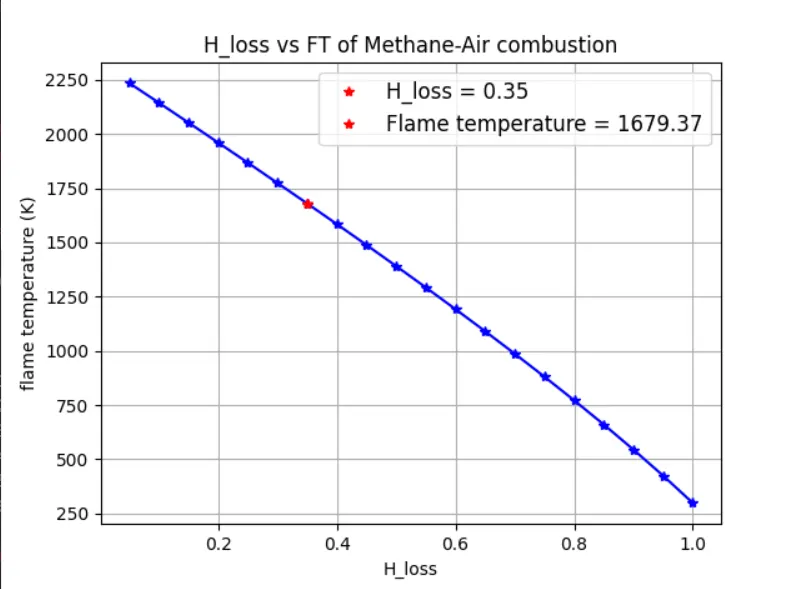
There is almost linear inverse relation between H_loss and Flame temperature. At H_loss = 0.35, Flame temperature is 1679.37 kelvin.
CASE-3 : Effect of bond structures of 2 carbon atom chains on AFT at constant pressure. Combustion is completely adiabatic. Results are compared to Cantera results. In cantera. we used constant Enthalpy and pressure to equilibrate the solution
Ethane has single bond C2H6
Ethene has double bond C2H4
Ethyne has triple bond C2H2
'''
Pyhton program for calculating the adiabatic flame temperature of 2 carbon atom chain with 3 different bond structures.

General Hydrocarbon reaction

CxHy + (x+y/4)(O2 + 3.76N2) = xCO2 + (y/2)H2O + (x+y/4)*3.76*N2

i> ethane = c2h6, consists of only single bonds

C2H6 + 3.5(O2 + 3.76N2) = 2CO2 + 3H20 + 13.16N2

ii> ethene = c2h4, consists of double bond

C2H4 + 3(O2 + 3.76N2) = 2CO2 + 2H20 + 11.26N2

iii> ethyne = c2h2, consists of triple bond

C2H2 + 2.5(O2 + 3.76N2) = 2CO2 + H20 + 9.40N2

Since the reaction is adiabatic there will not be any heat loss to the surrounding.

Reaction will take place at constant pressure.

Stochiometric reaction: Stoichiometric combustion occurs when all the oxygen is consumed in the reaction, and there is no molecular oxygen(O2) in the products.

'''
import matplotlib.pyplot as plt
import math
import cantera as ct
import numpy as np

R = 8.314 #j/mol-k
Tstd = 298.15

def h(T,co_effs):

	# function for evaluating enthalpy
	R = 8.314 #j/mol-k
	a1 = co_effs[0]
	a2 = co_effs[1]
	a3 = co_effs[2]
	a4 = co_effs[3]
	a5 = co_effs[4]
	a6 = co_effs[5]

	return (a1 + a2*T/2 + a3*pow(T,2)/3 +  a4*pow(T,3)/4 +  a5*pow(T,4)/5 + a6/T)*R*T

# Thermodata of the reactants at T<1000
c2h2_coeff_l = [8.08681094E-01,2.33615629E-02,-3.55171815E-05,2.80152437E-08,-8.50072974E-12,2.64289807E+04,1.39397051E+01]
c2h4_coeff_l = [3.95920148E+00,-7.57052247E-03,5.70990292E-05,-6.91588753E-08,2.69884373E-11,5.08977593E+03,4.09733096E+00]
c2h6_coeff_l = [4.29142492E+00,-5.50154270E-03,5.99438288E-05,-7.08466285E-08,2.68685771E-11,-1.15222055E+04,2.66682316E+00]
o2_coeff_l = [3.78245636E+00,-2.99673416E-03,9.84730201E-06,-9.68129509E-09,3.24372837E-12,-1.06394356E+03,3.65767573E+00]
n2_coeff_l = [0.03298677E+02,0.14082404E-02,-0.03963222E-04,0.05641515E-07,-0.02444854E-10,-0.10208999E+04,0.03950372E+02]

# Thermodata of the products at T>1000
n2_coeff_h = [0.02926640E+02,0.14879768E-02,-0.05684760E-05,0.10097038E-09,-0.06753351E-13,-0.09227977E+04,0.05980528E+02]
co2_coeff_h = [3.85746029E+00,4.41437026E-03,-2.21481404E-06,5.23490188E-10,-4.72084164E-14,-4.87591660E+04,2.27163806E+00]
h20_coeff_h = [3.03399249E+00,2.17691804E-03,-1.64072518E-07,-9.70419870E-11,1.68200992E-14,-3.00042971E+04,4.96677010E+00]

def f(T,ftype):

	h_c2h2_r = h(Tstd,c2h2_coeff_l)
	h_c2h4_r = h(Tstd,c2h4_coeff_l)
	h_c2h6_r = h(Tstd,c2h6_coeff_l)
	h_o2_r = h(Tstd,o2_coeff_l)
	h_n2_r = h(Tstd,n2_coeff_l)

	h_co2_p = h(T,co2_coeff_h)
	h_h20_p = h(T,h20_coeff_h)
	h_n2_p = h(T,n2_coeff_h)

	if ftype == 1:
		x = 2
		y = 6
		h_fuel = h_c2h6_r

	elif ftype == 2:
		x = 2
		y = 4
		h_fuel = h_c2h4_r

	elif ftype == 3:
		x = 2
		y = 2
		h_fuel = h_c2h2_r


	H_reactants = h_fuel + (x+y/4)*h_o2_r + (x+y/4)*3.76*h_n2_r

	H_products = x*h_co2_p  + (y/2)*h_h20_p + (x+y/4)*3.76*h_n2_p


	return H_products - H_reactants

def fprime(T,ftype):
	return (f(T+1e-6,ftype) - f(T,ftype))/(1e-6)

'''
performing newton-rhapson iteration

'''

alpha = 0.5
tol = 1e-3
ftype = [1,2,3]
AFT_py = []

for i in range(0,len(ftype)):
	T_guess = 1500
	while abs(f(T_guess,ftype[i])) > tol:
		T_guess = T_guess - alpha*(f(T_guess,ftype[i])/fprime(T_guess,ftype[i]))
	AFT_py.append(T_guess)
print(AFT_py)

plt.bar(['ethane','ethene','ethyne'],AFT_py)
plt.ylabel('Adiabatic flame temperature (K)')
plt.legend(fontsize = 12)
plt.title('ftype vs AFT')
plt.show()
# Adiabatic flame temperature obtained by using Cantera library.

gas = ct.Solution('gri30.xml')
AFT_ct = []
for i in range(0,len(ftype)):

	if ftype[i] == 1:
		x = 2
		y = 6
		fuel = 'C2H6'

	elif ftype[i] == 2:
		x = 2
		y = 4
		fuel = 'C2H4'

	elif ftype[i] == 3:
		x = 2
		y = 2
		fuel = 'C2H2'

	N_tot = 1 + (x+y/4) + 3.76*(x+y/4)
	N_fuel = 1/N_tot
	N_o2 = (x+y/4)/N_tot
	N_n2 = (3.76*(x+y/4))/N_tot

	# fuel-air properties
	gas.TPX = 298.15, 101325, {fuel :N_fuel,'O2':N_o2,'N2':N_n2}
	gas.equilibrate('HP','auto') # H = entalpy, P = pressure, auto = solver selection
	AFT_ct.append(gas.T)
print(AFT_ct)

plt.bar(['ethane','ethene','ethyne'],AFT_ct)
plt.ylabel('Adiabatic flame temperature (K)')
plt.legend(fontsize = 12)
plt.title('ftype vs AFT')
plt.show()

plt.plot(ftype,AFT_py,'-*',color='blue',label='Python')
plt.plot(ftype,AFT_ct,'-*',color='red',label='Cantera')
plt.xlabel('fuel type')
plt.ylabel('Adiabatic flame temperature (K)')
plt.legend(fontsize = 12)
plt.title('ftype vs AFT')
plt.show()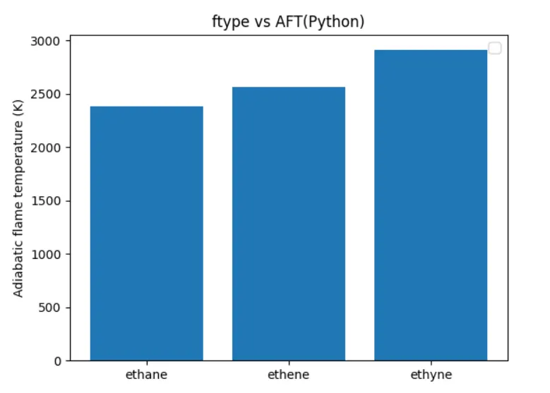
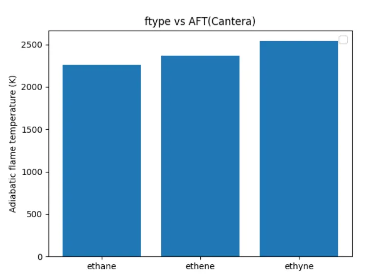
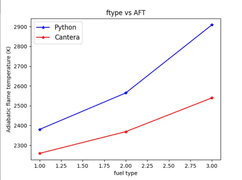
From the above graphs, it is to be observed that there is huge difference between AFT of ane,ene,yne fuels. As the bond strenght increased, the amount of heat generated was more which resulted in the increase of the temperature, This is due to the large amount of energy required to break the multi bonds. There is around 100 kelvin difference between the results obtained by python and cantera.
CASE-4 : For a general alkane, plotting the effect of the number of carbon atoms (from 1 to 3) on the final temperature. Assume H_loss = 0, Process will take place at constant pressure. Combustion is completely adiabatic. Results are compared to Cantera results. In cantera. we used constant Enthalpy and pressure to equilibrate the solution
'''
Pyhton program for calculating the adiabatic flame temperature of three different carbon chains.

General reaction

CxHy + (x+y/4)(O2 + 3.76N2) = xCO2 + (y/2)H2O + (x+y/4)*3.76*N2

i> methane = ch4.

CH4 + 2(O2 + 3.76N2) = CO2 + 2H20 + 7.52n2

ii> ethane = c2h6.

C2H6 + 3.5(O2 + 3.76N2) = 2CO2 + 3H20 + 13.16N2

iii> propane = c3h8, consists of triple bond

C3H8 + 5(O2 + 3.76N2) = 3CO2 + 4H20 + 18.8N2

Since the reaction is adiabatic there will not be any heat loss to the surrounding.

Reaction will take place at constant pressure.

Stochiometric reaction: Stoichiometric combustion occurs when all the oxygen is consumed in the reaction, and there is no molecular oxygen(O2) in the products.

'''
import matplotlib.pyplot as plt
import math
import cantera as ct
import numpy as np

R = 8.314 #j/mol-k
Tstd = 298.15

def h(T,co_effs):

	# function for evaluating enthalpy
	R = 8.314 #j/mol-k
	a1 = co_effs[0]
	a2 = co_effs[1]
	a3 = co_effs[2]
	a4 = co_effs[3]
	a5 = co_effs[4]
	a6 = co_effs[5]

	return (a1 + a2*T/2 + a3*pow(T,2)/3 +  a4*pow(T,3)/4 +  a5*pow(T,4)/5 + a6/T)*R*T

# Thermodata of the reactants at T<1000
ch4_coeff_l = [5.14987613E+00,-1.36709788E-02,4.91800599E-05,-4.84743026E-08,1.66693956E-11,-1.02466476E+04,-4.64130376E+00]
c2h6_coeff_l = [4.29142492E+00,-5.50154270E-03,5.99438288E-05,-7.08466285E-08,2.68685771E-11,-1.15222055E+04,2.66682316E+00]
c3h8_coeff_l = [0.93355381E+00,0.26424579E-01,0.61059727E-05,-0.21977499E-07,0.95149253E-11,-0.13958520E+05,0.19201691E+02]
o2_coeff_l = [3.78245636E+00,-2.99673416E-03,9.84730201E-06,-9.68129509E-09,3.24372837E-12,-1.06394356E+03,3.65767573E+00]
n2_coeff_l = [0.03298677E+02,0.14082404E-02,-0.03963222E-04,0.05641515E-07,-0.02444854E-10,-0.10208999E+04,0.03950372E+02]

# Thermodata of the products at T>1000
n2_coeff_h = [0.02926640E+02,0.14879768E-02,-0.05684760E-05,0.10097038E-09,-0.06753351E-13,-0.09227977E+04,0.05980528E+02]
co2_coeff_h = [3.85746029E+00,4.41437026E-03,-2.21481404E-06,5.23490188E-10,-4.72084164E-14,-4.87591660E+04,2.27163806E+00]
h20_coeff_h = [3.03399249E+00,2.17691804E-03,-1.64072518E-07,-9.70419870E-11,1.68200992E-14,-3.00042971E+04,4.96677010E+00]

def f(T,ftype):

	h_ch4_r = h(Tstd,ch4_coeff_l)
	h_c2h6_r = h(Tstd,c2h6_coeff_l)
	h_c3h8_r = h(Tstd,c3h8_coeff_l)
	h_o2_r = h(Tstd,o2_coeff_l)
	h_n2_r = h(Tstd,n2_coeff_l)

	h_co2_p = h(T,co2_coeff_h)
	h_h20_p = h(T,h20_coeff_h)
	h_n2_p = h(T,n2_coeff_h)

	if ftype == 1:
		x = 1
		y = 4
		h_fuel = h_ch4_r

	elif ftype == 2:
		x = 2
		y = 6
		h_fuel = h_c2h6_r

	elif ftype == 3:
		x = 3
		y = 8
		h_fuel = h_c3h8_r


	H_reactants = h_fuel + (x+y/4)*h_o2_r + (x+y/4)*3.76*h_n2_r

	H_products = x*h_co2_p  + (y/2)*h_h20_p + (x+y/4)*3.76*h_n2_p


	return H_products - H_reactants

def fprime(T,ftype):
	return (f(T+1e-6,ftype) - f(T,ftype))/(1e-6)

'''
performing newton-rhapson iteration

'''

alpha = 0.2
tol = 1e-3
ftype = [1,2,3]
AFT_py = []

for i in range(0,len(ftype)):
	T_guess = 1500
	while abs(f(T_guess,ftype[i])) > tol:
		T_guess = T_guess - alpha*(f(T_guess,ftype[i])/fprime(T_guess,ftype[i]))
	AFT_py.append(T_guess)
print(AFT_py)

plt.bar(['methane','ethane','propane'],AFT_py)
plt.ylabel('Adiabatic flame temperature (K)')
plt.legend(fontsize = 12)
plt.title('ftype vs AFT(Python)')
plt.show()
# Adiabatic flame temperature obtained by using Cantera library.

gas = ct.Solution('gri30.xml')
AFT_ct = []
for i in range(0,len(ftype)):

	if ftype[i] == 1:
		x = 1
		y = 4
		fuel = 'CH4'

	elif ftype[i] == 2:
		x = 2
		y = 6
		fuel = 'C2H6'

	elif ftype[i] == 3:
		x = 3
		y = 8
		fuel = 'C3H8'

	N_tot = 1 + (x+y/4) + 3.76*(x+y/4)
	N_fuel = 1/N_tot
	N_o2 = (x+y/4)/N_tot
	N_n2 = (3.76*(x+y/4))/N_tot

	# fuel-air properties
	gas.TPX = 298.15, 101325, {fuel :N_fuel,'O2':N_o2,'N2':N_n2}
	gas.equilibrate('HP','auto') # enthalpy = internal energy, p = pressure, auto = solver selection
	AFT_ct.append(gas.T)
print(AFT_ct)

plt.bar(['methane','ethane','propane'],AFT_ct)
plt.ylabel('Adiabatic flame temperature (K)')
plt.legend(fontsize = 12)
plt.title('ftype vs AFT(Cantera)')
plt.show()

plt.plot(ftype,AFT_py,'-*',color='blue',label='Python')
plt.plot(ftype,AFT_ct,'-*',color='red',label='Cantera')
plt.xlabel('fuel type')
plt.ylabel('Adiabatic flame temperature (K)')
plt.legend(fontsize = 12)
plt.title('ftype(alkanes) vs AFT')
plt.show()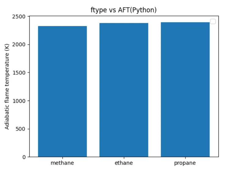
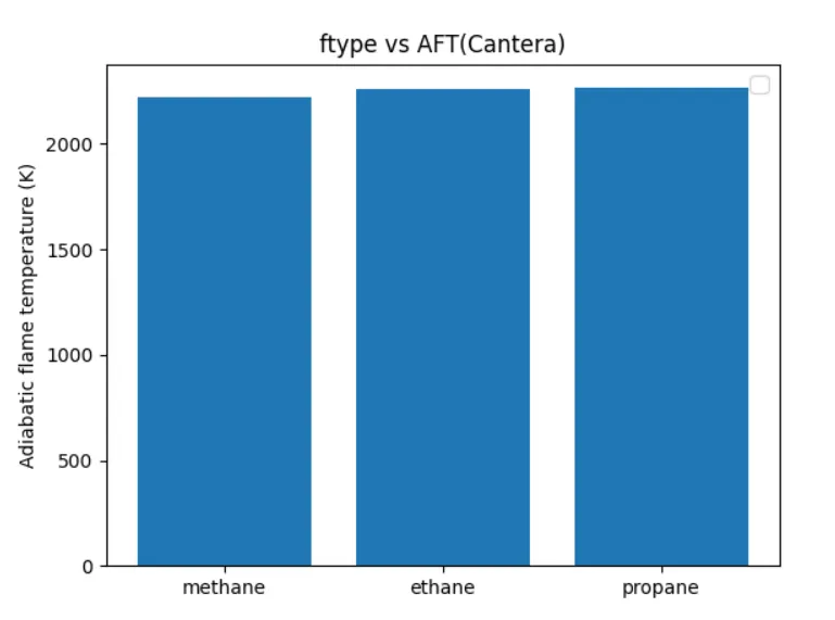
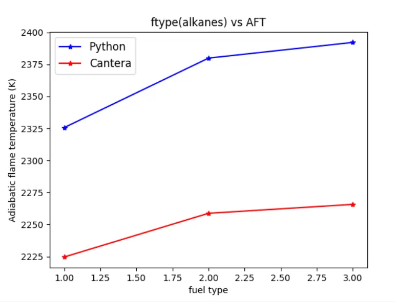
From above graphs and plots, it is evident that AFT does not vary much among different alkanes fuels as all the alkanes consists of single bonds in them. Python and Cantera results has a slight variation of 100 kelvin.