Week 3.5 - Deriving 4th order approximation of a 2nd order derivative using Taylor Table method
Deriving 4th order approximation of a 2nd order derivative using Taylor Table Method.
Taylor series formula is a representation of any function as an infinite sum of terms. These terms are calculated from the values of function’s derivatives at a single point. The derivative of a function f at the point x is defined as the limit of a difference quotient.
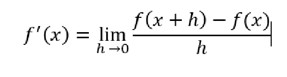
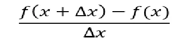
We can say the difference quotient is an approximation if the derivative f’(x) and its approximation gets better as h gets smaller. If h>0, say h = Dx where Dx is a finite positive number, then it is called the first-order or forward difference approximation of f’(x).
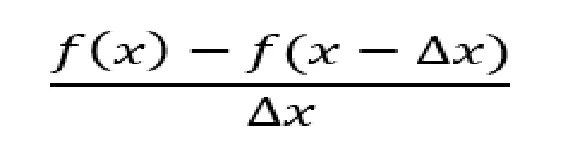
Similarly, if h<0, say h = -Dx, then the following expression is called as backward differencing approximation of f’(x).
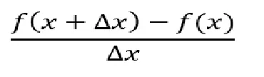
By combining different Taylor series expansions, we can obtain approximations of f’(x) of various orders. Second order centered difference approximations of second order derivative.
It is easy to calculate low order approximations. For higher order approximation we can use Taylor Table method. Taylor table contains coefficients of hypothesis and its derivative terms and it facilitates us to approximate function. Let us assume we want to find the fourth order approximation of second order derivative. For central differencing we have to take two forward and two backward point respective to point i .
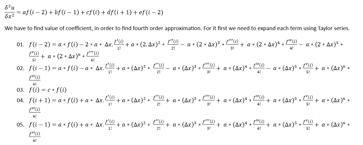
Taylor table can be generated as following.
|
|
|
Δ xfi’ |
Δx2 fi’’ |
Δx3 fi’’’ |
Δx4 fiiv |
Δx5 fiv |
Δx6 fivi |
|
af(i-2) |
a |
-2a |
4a/2 |
-8a/6 |
16a/24 |
-32a/120 |
64a/720 |
|
bf(i-1) |
b |
-b |
b/2 |
-b/6 |
b/24 |
-b/120 |
b/720 |
|
cfi |
c |
0 |
0 |
0 |
0 |
0 |
0 |
|
df(i+1) |
d |
d |
d/2 |
d/6 |
d/24 |
d/120 |
d/720 |
|
ef(i+2) |
e |
2e |
4e/2 |
8e/6 |
16e/24 |
32e/120 |
64e/720 |
|
∑ |
0 |
0 |
1 |
0 |
0 |
? |
? |
From the table equations of coefficient can be written as-
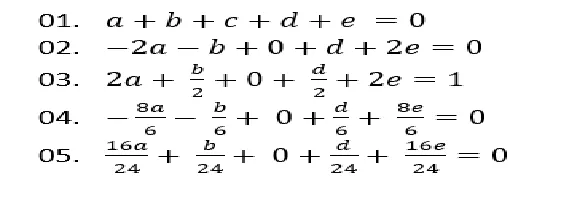
Matlab Code –
A = [1,1,1,1,1;-2,-1,0,1,2;2,1/2,0,1/2,2;-8/6,-1/6,0,1/6,8/6;16/24,1/24,0,1/24,16/24]
B = [0;0;1;0;0]
C = A\B
Result –
C =
-0.0833
1.3333
-2.5000
1.3333
-0.0833
Taylor table for Forward Differencing –
For forward differencing we have to selected four points forward to centre point those are i+1, i+2, i+3, i+4 and Taylor table can be generated in similar fashion as we did in central differencing.
|
|
Δ xfi’ |
Δx2 fi’’ |
Δx3 fi’’’ |
Δx4 fiiv |
Δx5 fiv |
Δx6 fivi |
||
|
af(i) |
a |
0 |
0 |
0 |
0 |
0 |
0 |
|
|
bf(i+1) |
b |
b |
b/2 |
b/6 |
b/24 |
b/120 |
b/720 |
|
|
cf(i+2) |
c |
2c |
2c |
8c/6 |
16c/24 |
32c/120 |
64c/720 |
|
|
df(i+3) |
d |
3d |
9d/2 |
27d/6 |
81d/24 |
243d/120 |
729d/720 |
|
|
ef(i+4) |
e |
4e |
16e/2 |
64e/6 |
256e/24 |
1024e/120 |
4096e/720 |
|
|
gf(i+5) |
g |
5g |
25g/2 |
125g/6 |
625g/24 |
3125g/120 |
15625g/720 |
|
|
∑ |
0 |
0 |
1 |
0 |
0 |
? |
? |
|
From the table equations of coefficient can be written as –
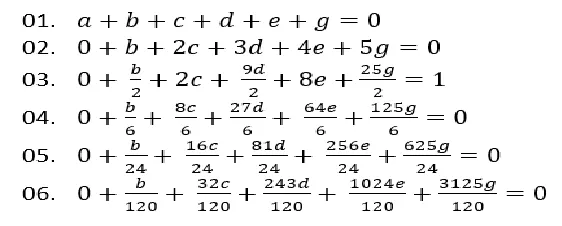
Matlab Code –
a = [1 1 1 1 1 1; 0 1 2 3 4 5; 0 1/2 2 9/2 16/2 25/2; 0 1/6 8/6 27/6 64/6 125/6; 0 1/24 16/24 81/24 256/24 625/24; 0 1/120 32/120 243/120 1024/120 3125/120];
b = [0;0;1;0;0;0];
c = a\b
Result –
c =
3.7500
-12.8333
17.8333
-13.0000
5.0833
-0.8333
Equation for second order with fourth order equation will be –

Taylor table for Backward differencing –
Point selected i, i-1, i-2, i-3, i-4
|
fi |
Δ xfi’ |
Δx2 fi’’ |
Δx3 fi’’’ |
Δx4 fiiv |
Δx5 fiv |
Δx6 fivi |
|
|
af(i) |
a |
0 |
0 |
0 |
0 |
0 |
0 |
|
bf(i-1) |
b |
-b |
b/2 |
-b/6 |
b/24 |
-b/120 |
b/720 |
|
cf(i-2) |
c |
-2c |
2c |
-8c/6 |
16c/24 |
-32c/120 |
64c/720 |
|
df(i-3) |
d |
-3d |
9d/2 |
-27d/6 |
81d/24 |
-243d/120 |
729d/720 |
|
ef(i-4) |
e |
-4e |
16e/2 |
-64e/6 |
256e/24 |
-1024e/120 |
4096e/720 |
|
gf(i-5) |
g |
-5g |
25g/2 |
-125g/6 |
625g/24 |
-3125g/120 |
15625g/720 |
|
∑ |
0 |
0 |
1 |
0 |
0 |
? |
? |
From the table equations of coefficient can be written as-
Equation for Second order with fourth order equation will be -

Code to find second order derivative and its fourth order derivative approximation.
Central, Right, Left Side differencing Function.
function [out1,out2,out3] = central_right_left_differenting(x,dx);
analytical_derivative = -2*exp(x)*sin(x);
numerical_derivative_central = (-0.0833.*exp(x-2.*dx).*cos(x-2.*dx)+1.3333.*exp(x-dx).*cos(x-dx)-2.5.*exp(x).*cos(x)+1.3333.*exp(x+dx)-0.0833.*exp(x+2.*dx).*cos(x+2.*dx))./((dx).^2);
% error_central = abs(analytical_derivative - numerical_derivative_central)
numerical_drivative_right =(3.75.*exp(x).*cos(x)-12.8333.*exp(x+dx).*cos(x+dx)+17.8333.*exp(x+2.*dx).*cos(x+2.*dx)-13.*exp(x+3.*dx).*cos(x+3.*dx)+5.0833.*exp(x+4.*dx).*cos(x+4.*dx)-0.8333.*exp(x+5.*dx).*cos(x+5.*dx))./((dx).^2);
numerical_drivative_left =(3.75.*exp(x).*cos(x)-12.8333.*exp(x-dx).*cos(x-dx)+17.8333.*exp(x-2.*dx).*cos(x-2.*dx)-13.*exp(x-3.*dx).*cos(x-3.*dx)+5.0833.*exp(x-4.*dx).*cos(x-4.*dx)-0.8333.*exp(x-5.*dx).*cos(x-5.*dx))./((dx).^2);
out1 = abs(analytical_derivative - numerical_derivative_central);
out2 = abs(analytical_derivative - numerical_drivative_right)
out3 = abs(analytical_derivative - numerical_drivative_left)
end
Main Code –
clear all
close all
clc
x = pi/3;
dx = linspace(pi/4000,pi/40,20);
%-2*e^x*sinx
for i = 1:length(dx);
[error_central(i), error_right(i), error_left(i)] = central_right_left_differenting(x,dx(i));
end
figure(1)
loglog(dx,error_central,'r')
hold on
loglog(dx,error_left,'g')
hold on
loglog(dx,error_right,'B')
xlabel('range of dx')
ylabel('truncation error')
title('range of dx vs error')
hold off
legend('central error','right error','left error')
Code Explanation –
One common program has written to compute fourth order approximation, backward, forward, central.
01. Define the variable x and dx. Dx is grid size or we can say approximation distance between two nodes. Dx is defined with linspace which provides a range of data.
02. Define the coefficient a, b directly in the equation, to form a single function file.
03. Define variable analytical derivative to find second order derivative of given function.
04. Define the numerical derivative variable which is an equation. Define error, which is difference of analytic and numerical derivative.
05. Loglog command is used to make log plot in command window.
06. We got plot which has forward approximation values above than central and backward approximation values below than central approximation values, it validates the theory. We infer from the graph that as values of dx is increasing the values of error also increasing.
07. The order of accuracy = Number of nodes in stencil - order of derivative of one sided
08. The order of accuracy = 6 -2 = 4
09. so, it proves that our skewed schemes are fourth order accurate.
Conclusion -
Since the central difference approximation is superior to the forward difference approximation in terms of truncation error, it is not preferred not always. In some cases, for example convection-diffusion equations, central differencing of convective terms can lead to numerical instabilities and poor resolution of steep gradients. It is appropriate to use a forward difference at the right endpoints, a backward difference at the left endpoints and centred difference formulas for the interior points. In CFD we often have values of points on the boundary i.e. boundary conditions, so how can we start central approximation, because we don’t have knowledge of interior point. So skewed approximation has advantage here.