Week 3.5 - Deriving 4th order approximation of a 2nd order derivative using Taylor Table method

OBJECTIVE-3 →→ Describe why a skewed scheme is useful? What can a skewed scheme do that a CD scheme cannot?

suppose we have to find the heat transfer values at the end of a concrete wall. In that case we are restricted with grid points only to one side, i.e. either left or right. In that scenarios, we cannot go for central differencing, since symmetric nodes is not possible.

 Central Difference (CD): The central difference approximation is derived by using Taylor series expansions around the point ( x ) and subtracting them to eliminate lower-order terms. The general formula for a 4th order central difference approximation of the second derivative is:

f′′(x)≈12h2−f(x+2h)+16f(x+h)−30f(x)+16f(x−h)−f(x−2h)​

 Skewed Right-Sided Difference: For the skewed right-sided difference, we use Taylor series expansions around the point ( x ) but skewed to the right, meaning we use points ( x+h, x+2h, \ldots ) to derive the approximation.

 Skewed Left-Sided Difference: Similarly, for the skewed left-sided difference, we use points to the left of ( x ), such as ( x-h, x-2h, \ldots ).

1. Choose Points: Select a set of points around the point where you want to approximate the derivative. For a central difference scheme, you might choose symmetric points around the central point.

2. Taylor Series Expansion: Write out the Taylor series expansions for each of these points up to the order of accuracy you’re interested in (in this case, 4th order).

3. Form Equations: Form equations for the derivative based on the Taylor expansions, expressing the derivative as a combination of the function values at the chosen points.

4. Solve for Coefficients: Solve the system of equations to find the coefficients that will give you the desired derivative approximation.

Here’s a simplified example using a central difference scheme for a 4th order approximation of the second derivative ( f’'(x) ):

Let’s consider five points: ( x_{i-2}, x_{i-1}, x_i, x_{i+1}, x_{i+2} ). The Taylor series expansions for these points are:

f(xi−2​)=f(xi​)−2hf′(xi​)+2!(2h)2​f′′(xi​)−3!(2h)3​f′′′(xi​)+4!(2h)4​f′′′′(xi​)+O(h5)

f(xi−1​)=f(xi​)−hf′(xi​)+2!h2​f′′(xi​)−3!h3​f′′′(xi​)+4!h4​f′′′′(xi​)+O(h5)

f(xi+1​)=f(xi​)+hf′(xi​)+2!h2​f′′(xi​)+3!h3​f′′′(xi​)+4!h4​f′′′′(xi​)+O(h5)

f(xi+2​)=f(xi​)+2hf′(xi​)+2!(2h)2​f′′(xi​)+3!(2h)3​f′′′(xi​)+4!(2h)4​f′′′′(xi​)+O(h5)

We want to find coefficients ( a, b, c, d, e ) such that:

a⋅f(xi−2​)+b⋅f(xi−1​)+c⋅f(xi​)+d⋅f(xi+1​)+e⋅f(xi+2​)=f′′(xi​)

Substitute the Taylor expansions into this equation and equate the coefficients of like powers of ( h ) to form a system of equations. Solve this system to find the values of ( a, b, c, d, e ) that will give you the second derivative to fourth-order accuracy.

CODE EXPLANATION:

Each scheme is coded in the form of 'function'.

The equation for all the schemes were solved initially on paper and in order to obtain the coefficients of the equation, they were solved using MATLAB (you can see in code).

It will ask user to input the value of x and range for dx respectively and these values are supplied to the function. After solving the function, the function itself is called in the main code.

The main code will give the comparison of the errors of all the schemes.

THEORY EXPLANATION:

The idea behinde using central, right hand skewed and left hand skewed schemes is to obtiain higher order approximation at the nodes which do not have left or right point (they are starting point).

Therefore, one can get the higher order approximation using right hand and left hand scheme.

HOW TO DECIDE NODES IN TAYLOR SERIES:

For skewed scheme, Number of nodes = order of derivative + order of approximation. In our case, order of derivative is 2nd order and order of approximation is 4th order. Therefore, Number of node = 2+4=6.

For central scheme, Number of nodes = order of derivative + order of approximation -1.In our case, order of derivative is 2nd order and order of approximation is 4th order. Therefore, Number of node = 2+4-1=5.

For right hand skew, [af(i)+bf(i+1)+cf(i+2)+df(i+3)+ef(i+4)+gf(i+5)]/(dx^2) (in our case)

For left hand skew, [af(i-5)+bf(i-4)+cf(i-3)+df(i-2)+ef(i-1)+gf(i)]/(dx^2) (in our case)

For central scheme, [af(i-2)+bf(i-1)+cf(i)+df(i+1)+ef(i+2)]/(dx^2) (in our case)

Initially, one must calculate the coefficients and then solve the equations.

COMPARISON →→

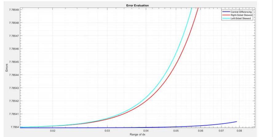
you can see in the above plots, the error is more for skewed schemes than for the central differencing schemes.

the errors, skewed left sided has started from 4.92⋅10−44.92⋅10-4, for central differencing - 4.935⋅10−44.935⋅10-4 and for the right sided scheme- 4.955⋅10−44.955⋅10-4. By the end of the curves, the error for central differencing is low and mostly linear, as comared to the skewed schems.

the large error values for skewed schemes than for the central differencing is because the no: of nodes is only 2-points apart, whereas in the skewed schemes, it is 5-points apart.

as the dx value reaches 1 or exceeds 1, then the error values will become unstable and the variations will much more.

also, the slope values of CD is less than the skewed schems. It means as the dx progresses, the frequency of error formation across the y-axis is constant. hence we get a linear plot and a minimum slope value.

%%---- CENTRAL SCHEME ----%%

% Function for 4th ORDER APPROX OF 2nd ORDER DERIVATIVE

% function = exp(x)*cos(x)

% analytical_derivative = - exp(x)*sin(x) + exp(x)*cos(x)

% CODE

function output = four_two_central(x,dx) % central

% For central scheme coefficient calculation

a1 =[1 1 1 1 1; -2 -1 0 1 2; 2 1/2 0 1/2 2; -8/6 -1/6 0 1/6 8/6; 16/24 1/24 0 1/24 16/24];

b1=[0; 0; 1; 0; 0];

coeff= linsolve(a1,b1);

% Analytical Solution

% analytical_derivative = (exp(x) * (cos(x)-sin(x)));

analytical_derivative = -2*(exp(x) * (sin(x)));

% Numerical Solution

a = ((exp(x-(2*dx))).*(cos(x-(2*dx))));

b = ((exp(x-dx)).*(cos(x-dx)));

c = (exp(x).*cos(x));

d = ((exp(x+dx)).*(cos(x+dx)));

e = ((exp(x+(2*dx))).*(cos(x+(2*dx))));

fourth_numerical_central = (((coeff(1))*a)+((coeff(2))*b)+((coeff(3))*c)+((coeff(4))*d)+(((coeff(5))*e)))/(dx.^2);

% Error

output = abs(fourth_numerical_central - analytical_derivative);

end

%%---- RIGHT HAND SCHEME ----%%

% Function for 4th ORDER APPROX OF 2nd ORDER DERIVATIVE

% function = exp(x)*cos(x)

% analytical_derivative = - exp(x)*sin(x) + exp(x)*cos(x)

% CODE

function output = fourth_forward_skew(x,dx) % (right hand side)

% For forward skewed scheme coefficient calculation (right hand side)

c1 = [1 1 1 1 1 1; 0 1 2 3 4 5; 0 1/2 2 9/2 8 25/2; 0 1/6 8/6 27/6 64/6 125/6; 0 1/24 16/24 81/24 256/24 625/24; 0 1/120 32/120 243/120 1024/120 3125/120];

d1 = [0; 0; 1; 0; 0; 0];

coeff= linsolve(c1,d1);

% Analytical Solution

% analytical_derivative = (exp(x) * (cos(x)-sin(x)));

analytical_derivative = -2*(exp(x) * (sin(x)));

% Numerical Solution

p= (exp(x)*cos(x));

q= ((exp(x+dx)).*(cos(x+dx)));

r= ((exp(x+(2*dx))).*(cos(x+(2*dx))));

s= ((exp(x+(3*dx))).*(cos(x+(3*dx))));

t= ((exp(x+(4*dx))).*(cos(x+(4*dx))));

u= ((exp(x+(5*dx))).*(cos(x+(5*dx))));

forward_skew = (((15/4)*p)+((-77/6)*(q))+((107/6)*(r))+((-13)*(s))+((61/12)*(t))+((-5/6)*(u)))/(dx.^2);

% Error

output = abs(forward_skew - analytical_derivative);

end

%%---- LEFT HAND SCHEME---- %%

% Function for 4th ORDER APPROX OF 2nd ORDER DERIVATIVE

% function = exp(x)*cos(x)

% analytical_derivative = - exp(x)*sin(x) + exp(x)*cos(x)

% CODE

function output = fourth_backward_skew(x,dx) % Left hand side

% For backward skewed scheme coefficient calculation (left hand side)

l1 = [1 1 1 1 1 1; -5 -4 -3 -2 -1 0; 25/2 16/2 9/2 4/2 1/2 0; -125/6 -64/6 -27/6 -8/6 -1/6 0; 625/24 256/24 81/24 16/24 1/24 0; -3125/120 -1024/120 -243/120 -32/120 -1/120 0];

m1 = [0; 0; 1; 0; 0; 0];

coeff= linsolve(l1,m1);

% Analytical Solution

% analytical_derivative = (exp(x) * (cos(x)-sin(x)));

analytical_derivative = -2*(exp(x) * (sin(x)));

% Numerical Solution

a= ((exp(x-(5*dx))).*(cos(x-(5*dx))));

b= ((exp(x-(4*dx))).*(cos(x-(4*dx))));

c= ((exp(x-(3*dx))).*(cos(x-(3*dx))));

d= ((exp(x-(2*dx))).*(cos(x-(2*dx))));

e= ((exp(x-(dx))).*(cos(x-(dx))));

g= ((exp(x))*(cos(x)));

backward_skew = ((-5/6*(a))+(61/12*(b))+(-13*(c))+(107/6*(d))+(-77/6*(e))+(15/4*(g)))/(dx.^2);

% Error

output = abs(backward_skew - analytical_derivative);

end

%%---- MAIN CODE ----%%

% Main Code

n = input('Specify Value of x: ');

m = input('Input start value of dx: ');

o = input('Input end value of dx: ');

p = input('Input number of points: ');

x= n;

dx= linspace(m,o,p);

% Analytical Solution

analytical_derivative = (exp(x) * (cos(x)-sin(x)));

% For loop for ERROR calculation

for i = 1:length(dx)

central_error(i) = four_two_central(x,dx(i));

forward_skew_error(i) = fourth_forward_skew(x,dx(i));

backward_skew_error(i) = fourth_backward_skew(x,dx(i));

end

% Plotting

figure(1)

loglog(dx,central_error,'r')

hold on

loglog(dx,forward_skew_error,'g')

hold on

loglog(dx,backward_skew_error,'b')

xlabel('dx')

ylabel('Error')

grid on;

legend('Central Error','Forward Error','Backward Error')