Week 3.5 - Deriving 4th order approximation of a 2nd order derivative using Taylor Table method

Function Code:

function [error_CD] = central_diffrencing(x,dx,x_CD)
%anonymous function
f=@(x) exp(x).*cos(x)
%analytical derrivative
analytical_derrivative = -2*exp(x)*sin(x)
%central diffrencing
central_diffrencing_approx = (x_CD(1).*f(x-2.*dx)+x_CD(2).*f(x-dx)+x_CD(3).*f(x)+x_CD(4).*f(x+dx)+x_CD(5).*f(x+2.*dx))./(dx.^2);
%error calculation
error_CD = abs(central_diffrencing_approx-analytical_derrivative)
end

function [error_RH] = right_hand_scheme(x,dx,x_RH)
%anonymous function
f=@(x) exp(x).*cos(x)
%analytical derrivative
analytical_derrivative = -2*exp(x)*sin(x)
%right hand scheme 
right_hand_scheme = (x_RH(1).*f(x)+x_RH(2).*f(x+dx)+x_RH(3).*f(x+2.*dx)+x_RH(4).*f(x+3.*dx)+x_RH(5).*f(x+4.*dx)+x_RH(6).*f(x+5.*dx))./(dx.^2);
%error calculation
error_RH = abs(right_hand_scheme-analytical_derrivative)
end

function [error_LH] = left_hand_scheme(x,dx,x_LH)
%anonymous function
f=@(x) exp(x).*cos(x)
%analytical derrivative
analytical_derrivative = -2*exp(x)*sin(x)
%left hand scheme 
left_hand_scheme = (x_LH(1).*f(x)+x_LH(2).*f(x-dx)+x_LH(3).*f(x-2.*dx)+x_LH(4).*f(x-3.*dx)+x_LH(5).*f(x-4.*dx)+x_LH(6).*f(x-5.*dx))./(dx.^2);
%error calculation
error_LH = abs(left_hand_scheme-analytical_derrivative)
end

Main Code:

clear all 
close all
clc

%inputs
x = pi/3;
dx = linspace(pi/4000,1.5*pi,20);

%finding the unknown coefficients 
%for  central diffrencing
A_CD = [1,1,1,1,1;-2,-1,0,1,2;2,1/2,0,1/2,2;-8/6,-1/6,0,1/6,8/6;16/24,1/24,0,1/24,16/24]
B_CD = [0;0;1;0;0]
x_CD = inv(A_CD)*B_CD

%for right hand scheme 
A_RH = [1,1,1,1,1,1;0,1,2,3,4,5;0,1/2,4/2,9/2,16/2,25/2;0,1/6,8/6,27/6,64/6,125/6;0,1/24,16/24,81/24,256/24,625/24;0,1/120,32/120,243/120,1024/120,3125/120]
B_RH = [0;0;1;0;0;0]
x_RH = inv(A_RH)*B_RH

%for left had scheme
A_LH = [1,1,1,1,1,1;0,-1,-2,-3,-4,-5;0,1/2,4/2,9/2,16/2,25/2;0,-1/6,-8/6,-27/6,-64/6,-125/6;0,1/24,16/24,81/24,256/24,625/24;0,-1/120,-32/120,-243/120,-1024/120,-3125/120]
B_LH = [0;0;1;0;0;0]
x_LH = inv(A_LH)*B_LH

%truncation error value computing 
%error in right hand scheme(when order of approximation is 4 and order of derrivative is 2)
[error_RH] = right_hand_scheme(x,dx,x_RH)
%error in left hand scheme(when order of approximation is 4 and order of derrivative is 2)
[error_CD] = central_diffrencing(x,dx,x_CD)
%error in central diffrencing (when order of approximation is 4 and order of derrivative is 2)
[error_LH] = left_hand_scheme(x,dx,x_LH)

%ploting 
figure(1)
loglog(dx,error_CD,LineWidth=2)
hold on
loglog(dx,error_LH,LineWidth=2)
loglog(dx,error_RH,LineWidth=2)
grid on
legend('central diffrencing','left hand scheme','right hand scheme')
xlabel('change in dx')
ylabel('truncation error')

Question:

Derive the following 4th order approximations of the second-order derivative.

1. Central difference
2. Skewed right-sided difference
3. Skewed left-sided difference

Objective:

1. After deriving these schemes, prove that your skewed schemes are fourth-order accurate
2. Once you have done this, write a program in MATLAB to evaluate the second-order derivative of the analytical function exp(x)*cos(x)and compare it with the 3 numerical approximations that you have derived.
3. Provide a plot that compares the absolute error between the above-mentioned schemes in your own words, describe why a skewed scheme is useful? What can a skewed scheme do that a CD scheme cannot?

Solution:

Deriving central differencing 4^th order approximation:

The order of accuracy(P) = number of nodes in stencil(N) - order of derivative(Q)+1

So, N = P + Q-1

N = 2 + 4 - 1

i-2 i-1 i i+1 i+2

`(∂^(2 ) u)/(∂x^2 )=(af(i-2)+bf(i-1)+cf(i)+df(i+1)+ef(i+2))/(dx^2 )` ……….. (1)

in above equation we need to find the coefficients a, b, c, d, e. by using Taylors expansion

for ex,

`af(i-2)=af(i)-(af(i)(2∆x))/(1!)+(af(i)4ax^2)/(2!)-(af(i)8ax^3)/(3!)………`

Using Taylors expansion, we get the Taylors table which we can see below;

	f(i)	∆xf’(x)	∆x2f’’(x)	∆x3f’’’(x)	∆x4f’’’’(x)	∆x5f’’’’’(x)	∆x6f’’’’’’(x)
af(i-2)	a	-2a	4a/2	-8a/6	16a/24	-32a/120	64a/240
bf(i-1)	b	-b	b/2	-b/6	b/24	-b/120	b/240
cf(i)	c	0	0	0	0	0	0
df(i+1)	d	d	d/2	d/6	d/24	d/120	d/240
ef(i+2)	e	2e	4e/2	8e/6	16e/24	32e/120	64e/240
	0	0	1	0	0

In above table row means value of term calculated by using Taylor series, and as we are solving for the 2^nd order rest of terms becomes 0, but we don’t know about 5^th and 6^th term and we don’t have any interest in knowing that as we have only 5 unknows and we got 5 equations for that;

`a+b+c+d+e=0`

`-2a-b+0+d/2+2e=0`

`2a+b/2+0+d/2+2e=1`

`(-8a)/6-b/6+d/6+(8e)/6=0`

`(16a)/24+b/24+0+d/24+(16e)/24=0`

Now form above set of equations we get the matrix ;

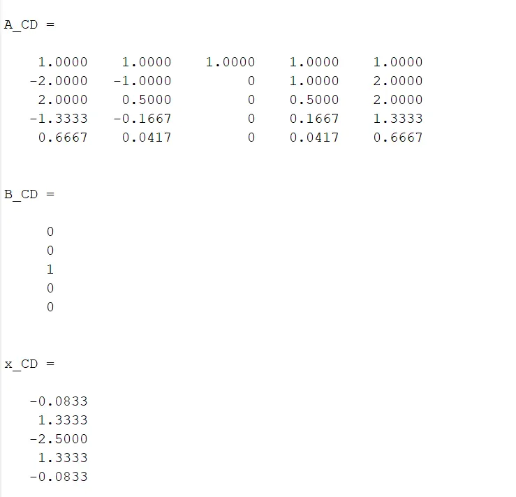
Which comes in form of A*X=B;

Where, X contains coefficients, so to find X we divide A/B

X=A/B;

By solving this we gets the X in form of 5x1 matrix,

So coefficient becomes, a=-0.8333, b=1.3333, c=-2.5000, d=1.3333, e=-0.8333

Now if we see e=a and b=d

After getting coefficients we substitute the values in equation 1 so we get central differencing equation ;

`(∂^2 u)/(∂x^2 )=(-0.8333f(i-2)+1.3333(i-1)-2.5000f(i)+1.3333f(i+1)-0.8333f(i+2))/(dx^2 )`

Now lets add all term from taylors table, af(i-2)+bf(i-2)+cf(i)+df(i+1)+ef(i+2)

`=(a+b+c+d+e)f(i)+(-2a-b+0+d+2e) f^' (x)∆x +(2a+b/2+0+d+2e) f^'' (x)∆x^2+(-(8a)/6-b/6+0+d/6+(8e)/6) f^''' (x)∆x^3 +((16a)/24+b/24+0+d/24+(16e)/24) f^'''' (x)∆x^4+((-32a)/120-b/120+0+d/120+(32e)/120) f^''''' (x)∆x^5 +((64a)/24+b/240+0+d/240+(64e)/240)f'''''''(x)∆x^6`

Now in above Taylors table we already cleared that only 2^nd order term is equal to 1 rest of terms are 0 except 5^th and 6^th order term

And if we replace a=e and b=d in 5^th term it also becomes zero

`af(i-2)+bf(i-2)+cf(i)+df(i+1)+ef(i+2)]=[(2a+b/2+0+d+2e) f^'' (x)∆x^2 +((64a)/24+b/240+0+d/240+(64e)/240)f'''''''(x)∆x^6`

Divide both side by ∆x²

`[af(i-2)+bf(i-2)+cf(i)+df(i+1)+ef(i+2)]/(∆x^2 )=[(2a…) f^'' (x)∆x^2+(….) f^'''''' (x)∆x^2 ]/(∆x^2 )`

We ignore the higher order term now so we can say that as truncation error

We get;

`[af(i-2)+bf(i-2)+cf(i)+df(i+1)+ef(i+2)]/(∆x^2 )=(2a….+2e) f^'' (x)+0(∆x^4 )`

`[af(i-2)+bf(i-2)+cf(i)+df(i+1)+ef(i+2)]/(∆x^2 )=(2a….+2e) f^'' (x)+0(∆x^4 )`

Now from above term if we can say that order of approximation is 4 of the 2^nd order derivatives

Skewed right hand difference scheme:

No of nodes = P + Q = 2+4=6

Where, P is order of derivative and Q is order of approximation

i i+1 i+2 i+3 i+4 i+5

`(∂^2 u)/(∂x^2 )=(af(i)+bf(i+1)+cf(i+2)+df(i+3)+ef(i+4)gf(i+5))/(dx^2 )`

using Taylors series the Taylors table we get is ;

	f(i)	∆xf’(x)	∆x2f’’(x)	∆x3f’’’(x)	∆x4f’’’’(x)	∆x5f’’’’’(x)
af(i)	a	0	0	0	0	0
bf(i+1)	b	b	b/2	b/6	b/24	b/120
cf(i+2)	c	2c	4c/2	8c/6	16c/24	32c/120
df(i+3)	d	3d	9d/2	27d/6	81d/24	243d/120
ef(i+4)	e	4e	16e/2	64e/6	256e/24	1024e/120
gf(i+5)	g	5g	25g/2	125g/6	625g/24	3125g/120
Sum of coefficients	0	0	1	0	0	0

The linear equations obtain from above table

`a+b+c+d+e+g=0`

`0+b+2c+3d+4e+5g=0`

`0+b/2+(4c)/2+(9d)/2+(16e)/2+(25g)/2=1`

`0+b/6+(8c)/6+(27d)/6+(64e)/6+(125g)/6=0`

`0+b/24+(16c)/24+(81d)/24+(256e)/24+(625g)/24=0`

`0+b/120+(32c)/120+(243d)/120+(1024e)/120+(3125g)/120=0`

Which gives us matrix, and results

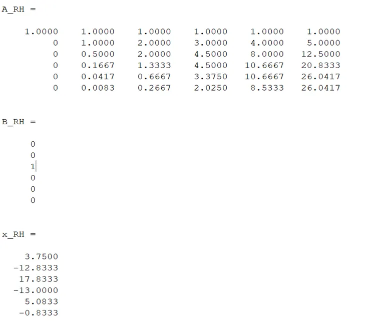
Hence the right-hand scheme equation becomes;

`(∂^2 u)/(∂x^2 )=(3.7500f(i)-12.8333f(i+1)+17.8333f(i+2)-13.0000f(i+3)+5.0833f(i+4)-0.8333f(i+5))/(dx^2 )`

Skewed Left hand difference scheme:

No of nodes = P + Q = 2+4=6

Where, P is order of derivative and Q is order of approximation

i-5 i-4 i-3 i-2 i-1 i

`(∂^2 u)/(∂x^2 )=(af(i)+bf(i-1)+cf(i-2)+df(i-3)+ef(i-4)+gf(i-5))/(dx^2 )`

using Taylors series the Taylors table we get is;

	f(i)	∆xf’(x)	∆x2f’’(x)	∆x3f’’’(x)	∆x4f’’’’(x)	∆x5f’’’’’(x)
af(i)	a	0	0	0	0	0
bf(i+1)	b	-b	b/2	-b/6	b/24	-b/120
cf(i+2)	c	-2c	4c/2	-8c/6	16c/24	-32c/120
df(i+3)	d	-3d	9d/2	-27d/6	81d/24	-243d/120
ef(i+4)	e	-4e	16e/2	-64e/6	256e/24	-1024e/120
gf(i+5)	g	-5g	25g/2	-125g/6	625g/24	-3125g/120
Sum of coefficients	0	0	1	0	0	0

linear equations are:

`a+b+c+d+e+g=0`

`0-b-2c-3d-4e-5g=0`

`0+b/2+(4c)/2+(9d)/2+(16e)/2+(25g)/2=1`

`0-b/6-(8c)/6-(27d)/6-(64e)/6-(125g)/6=0`

`0+b/24+(16c)/24+(81d)/24+(256e)/24+(625g)/24=0`

`0-b/120-(32c)/120-(243d)/120-(1024e)/120-(3125g)/120=0`

Using above equations, the matrix and coefficients value we get is;

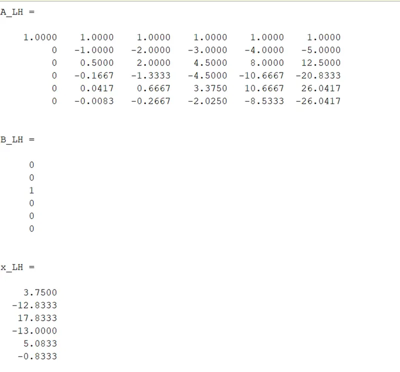
Hence the left-hand scheme equation becomes;

`(∂^2 u)/(∂x^2 )=(3.7500f(i)-12.8333f(i-1)+17.8333f(i-2)-13.0000f(i-3)+5.0833f(i-4)-0.8333f(i-5))/(dx^2 )`

Code explanation:

1. In code first of all We define the inputs x and dx, Were Dx is the range.
2. Up next we create a function code For all the three schemes (Left hand difference scheme, right hand difference scheme, and central differencing). Were while creating function we Take inputs x, dx and coefficient defined to the scheme respectively(for ex x_CD, x_RH and x_LH).
3. To solve this challenge here one Analytical function is given, f(x)=exp(x)*cos(x), so First, we take its second order derivative which becomes f’’(x)=-2*exp(x)*sin(x) and name it as analytical derivative After that we define the schemes equation which we created above using the Taylor series lets take example of central differencing;

central_diffrencing_approx = (x_CD(1).*f(x-2.*dx)+x_CD(2).*f(x-dx)+x_CD(3).*f(x)+x_CD(4).*f(x+dx)+x_CD(5).*f(x+2.*dx))./(dx.^2);

here x_CD(1) means 1^st row of matrix x_CD which we created using above derivations likewise;

x_CD(1) =a, x_CD(2)=b, x_CD(3)=c, x_CD(4)=d, x_CD(5)=e;

and for f(x) we define function using the anonymous function; f=@(x) exp(x)*cos(x)

4. now using above procedure we creat the all 3 schemes function and now its time to apply that in main code by calling all the three functions:

[error_RH] = right_hand_scheme(x,dx,x_RH)

[error_CD] = central_diffrencing(x,dx,x_CD)

[error_LH] = left_hand_scheme(x,dx,x_LH)

5. as of now we get all the numbers so lets plot dx vs error using set of plotting commands

Results:

As a result we get the plot of dx vs error values we get from various schemes

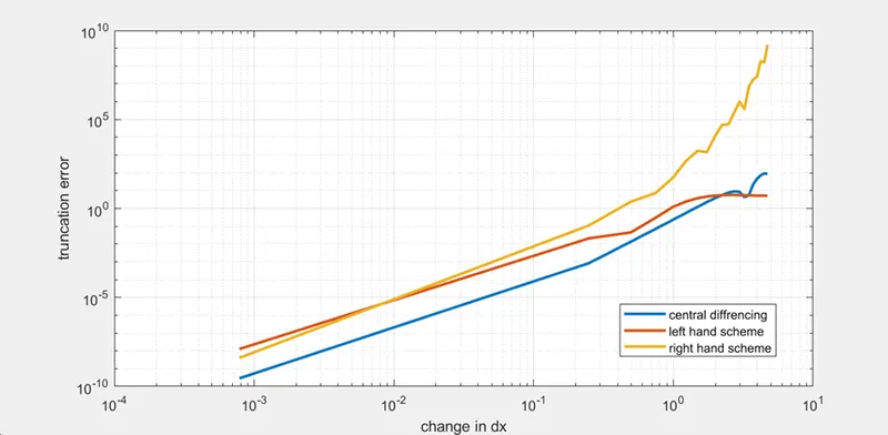
Fig 1. Dx vs Truncation error

Why skewed scheme is useful and what it provides which central differencing cannot?

Skewed scheme is useful because every time we will not get the sufficient information from both sides so during such type of cases we use skewed schemes this type of scheme is useful near the boundary conditions where we can’t imply the central differencing and that’s the thing which central differencing cannot provide.