Week 3.5 - Deriving 4th order approximation of a 2nd order derivative using Taylor Table method

Objective:

• To derive the fourth order approximation of second order derivative using central difference, skewed right-sided difference and skewed left-sided difference methods.
• To find the second order derivative of the given analytical function using the above derived formulae and compute the errors in each case using Matlab. Also, plot a comparison graph for the same.
  • Analytical Function: `f(x)=e^x*cosx`
    • Conditions: `x=pi/3;dx=[pi/400...<"20 Values">...pi/40]`
• To elaborate the significance of a skewed scheme over a central scheme.

Derivation:

• Central Difference Method:
  • To find the number of nodes required to compute the fourth order approximation of the second order derivative using central difference scheme, the following formula is used:
    • `"No. of nodes(N) "=" Order of the derivative(p)"+"Order of approximation(q)"-1`
    • Here, `p=2; q=4=>N=2+4-1=bb5`
  • So, five nodes are required to compute it, i.e., 4 nodes in addition to the point at which the derivative is to be found. As it is central difference scheme, 2 nodes before and 2 nodes after the reference point. Simply, the nodes are (i-2), (i-1), i, (i+1), (i+2).
  • Therefore the hypothesis function is:
    • `=>Deltax^2*(d^2u)/dx^2=a*f(i-2)+b*f(i-1)+c*f(i)+d*f(i+1)+e*f(i+2)`
  • Taylor's Table:

    • `Deltax^2*(d^2u)/dx^2`	`f(i)`	`Deltax*f'(i)`	`Deltax^2*f"''"(i)`	`Deltax^3*f"'''"(i)`	`Deltax^4*f^"iv"(i)`
      `a*f(i-2)`	`a`	`-2*a`	`(4*a)/2`	`-(8*a)/6`	`(16*a)/24`
      `b*f(i-1)`	`b`	`-b`	`b/2`	`-b/6`	`b/24`
      `c*f(i)`	`c`	`0`	`0`	`0`	`0`
      `d*f(i+1)`	`d`	`d`	`d/2`	`d/6`	`d/24`
      `e*f(i+2)`	`e`	`2*e`	`(4*e)/2`	`(8*e)/6`	`(16*e)/24`
      Adding the above: `Deltax^2*(d^2u)/dx^2`	`darr` `0`	`darr` `0`	`darr` `1`	`darr` `0`	`darr` `0`

  • By solving(using Matlab) the above equations, the value of a,b,c,d and e can be found.
  • So, the formula for the central differencing scheme is:
    • `=>Deltax^2*(d^2u)/dx^2=-0.0833*f(i-2)+1.3333*f(i-1)-2.5*f(i)+1.3333*f(i+1)-0.0833*f(i+2)`
    • `=>((d^2u)/dx^2)_("Central Diff")=(-0.0833*f(i-2)+1.3333*f(i-1)-2.5*f(i)+1.3333*f(i+1)-0.0833*f(i+2))/(Deltax^2)`

• Skewed Right-sided Difference Method:
  • Again, to find the number of nodes required to compute the fourth order approximation of the second order derivative using skewed right-sided difference scheme, the following formula is used:
    • `"No. of nodes(N) "=" Order of the derivative(p)"+"Order of approximation(q)"-1`
    • Here, `p=2; q=4=>N=2+4=bb6`
  • So, six nodes are required to compute it, i.e., 5 nodes in addition to the point at which the derivative is to be found. As it is skewed right-sided difference scheme, 5 nodes after the reference point is taken. Simply, the nodes are i,(i+1), (i+2), (i+3), (i+4), (i+5).
  • Therefore the hypothesis function is:
    • `=>Deltax^2*(d^2u)/dx^2=a*f(i)+b*f(i+1)+c*f(i+2)+d*f(i+3)+e*f(i+4)+g*f(i+5)`
  • Taylor's Table:

    • `Deltax^2*(d^2u)/dx^2`	`f(i)`	`Deltax*f'(i)`	`Deltax^2*f"''"(i)`	`Deltax^3*f"'''"(i)`	`Deltax^4*f^"iv"(i)`	`Deltax^5*f^"v"(i)`
      `a*f(i)`	`a`	`0`	`0`	`0`	`0`	`0`
      `b*f(i+1)`	`b`	`b`	`b/2`	`b/6`	`b/24`	`b/120`
      `c*f(i+2)`	`c`	`2*c`	`(4*c)/2`	`(8*c)/6`	`(16*c)/24`	`(32*c)/120`
      `d*f(i+3)`	`d`	`3*d`	`(9*d)/2`	`(27*d)/6`	`(81*d)/24`	`(243*d)/120`
      `e*f(i+4)`	`e`	`4*e`	`(16*e)/2`	`(64*e)/6`	`(256*e)/24`	`(1024*e)/120`
      `g*f(i+5)`	`g`	`5*g`	`(25*g)/2`	`(125*g)/6`	`(625*g)/24`	`(3125*g)/120`
      Adding the above: `Deltax^2*(d^2u)/dx^2`	`darr` `0`	`darr` `0`	`darr` `1`	`darr` `0`	`darr` `0`	`darr` `0`

  • Similarly, by solving(using Matlab) the above equations, the value of a, b, c, d, e and g can be found.
  • So, the formula for the skewed right-sided differencing scheme is:
    • `=>Deltax^2*(d^2u)/dx^2=3.7500*f(i)-12.8333*f(i+1)+17.8333*f(i+2)-13*f(i+3)+5.0833*f(i+4)-0.8333*f(i+5)`
    • `=>((d^2u)/dx^2)_("Skewed Right-sided Diff")=(3.7500*f(i)-12.8333*f(i+1)+17.8333*f(i+2)-13*f(i+3)+5.0833*f(i+4)-0.8333*f(i+5))/(Deltax^2)`

• Skewed Left-sided Difference Method:
  • Similar to that of the right-sided scheme, using the same formula, six nodes are required to compute it, i.e., 5 nodes in addition to the point at which the derivative is to be found. As it is skewed left-sided difference scheme, 5 nodes before the reference point is taken. Simply, the nodes are i, (i-1), (i-2), (i-3), (i-4), (i-5).
  • Therefore the hypothesis function is:
    • `=>Deltax^2*(d^2u)/dx^2=a*f(i)+b*f(i-1)+c*f(i-2)+d*f(i-3)+e*f(i-4)+g*f(i-5)`
  • Taylor's Table:

    • `Deltax^2*(d^2u)/dx^2`	`f(i)`	`Deltax*f'(i)`	`Deltax^2*f"''"(i)`	`Deltax^3*f"'''"(i)`	`Deltax^4*f^"iv"(i)`	`Deltax^5*f^"v"(i)`
      `a*f(i)`	`a`	`0`	`0`	`0`	`0`	`0`
      `b*f(i-1)`	`b`	`-b`	`b/2`	`-b/6`	`b/24`	`-b/120`
      `c*f(i-2)`	`c`	`-2*c`	`(4*c)/2`	`-(8*c)/6`	`(16*c)/24`	`-(32*c)/120`
      `d*f(i-3)`	`d`	`-3*d`	`(9*d)/2`	`-(27*d)/6`	`(81*d)/24`	`-(243*d)/120`
      `e*f(i-4)`	`e`	`-4*e`	`(16*e)/2`	`-(64*e)/6`	`(256*e)/24`	`-(1024*e)/120`
      `g*f(i-5)`	`g`	`-5*g`	`(25*g)/2`	`-(125*g)/6`	`(625*g)/24`	`-(3125*g)/120`
      Adding the above: `Deltax^2*(d^2u)/dx^2`	`darr` `0`	`darr` `0`	`darr` `1`	`darr` `0`	`darr` `0`	`darr` `0`

  • Similarly, by solving(using Matlab) the above equations, the value of a, b, c, d, e and g can be found.
  • So, the formula for the skewed left-sided differencing scheme is:
    • `=>Deltax^2*(d^2u)/dx^2=3.7500*f(i)-12.8333*f(i-1)+17.8333*f(i-2)-13*f(i-3)+5.0833*f(i-4)-0.8333*f(i-5)`
    • `=>((d^2u)/dx^2)_("Skewed Left-sided Diff")=(3.7500*f(i)-12.8333*f(i-1)+17.8333*f(i-2)-13*f(i-3)+5.0833*f(i-4)-0.8333*f(i-5))/(Deltax^2)`
• Proving Skewed scheme is of fourth order approximation:
  • Given Formula: `"Order of accuracy " P = "Number of nodes in the stencil "N - "order of derivative "Q`
  • Here, `N=6("as 6 nodes are taken to calculate"); Q=2 => P=6-2=bb4`
  • Hence, it's proved that the skewed scheme is of fourth order accuracy!

Matlab Program:

Main Program:

clear all
close all
clc

%Defining x and dx
x=pi/3;
dx=linspace(pi/400,pi/40,20);

%Finding Coefficients
%Skewed Right Sided Difference Coefficients
A_1=[1,1,1,1,1,1;
    0,1,2,3,4,5;
    0,1/2,4/2,9/2,16/2,25/2;
    0,1/6,8/6,27/6,64/6,125/6;
    0,1/24,16/24,81/24,256/24,625/24;
    0,1/120,32/120,243/120,1024/120,3125/120];
B_1=[0;0;1;0;0;0];
X_1=inv(A_1)*B_1

%Skewed Left Sided Difference Coefficients
A_2=[1,1,1,1,1,1;
    0,-1,-2,-3,-4,-5;
    0,1/2,4/2,9/2,16/2,25/2;
    0,-1/6,-8/6,-27/6,-64/6,-125/6;
    0,1/24,16/24,81/24,256/24,625/24;
    0,-1/120,-32/120,-243/120,-1024/120,-3125/120];
B_2=[0;0;1;0;0;0];
X_2=inv(A_2)*B_2

%Central Difference Coefficients
A_3=[1,1,1,1,1;
    -2,-1,0,1,2;
    4/2,1/2,0,1/2,4/2;
    -8/6,-1/6,0,1/6,8/6;
    16/24,1/24,0,1/24,16/24];
B_3=[0;0;1;0;0];
X_3=inv(A_3)*B_3

%Finding Error
for i=1:length(dx)
    error_skewed_right_sided(i)=Skewed_Right_Sided(x,dx(i),X_1);
    error_skewed_left_sided(i)=Skewed_Left_Sided(x,dx(i),X_2);
    error_central(i)=Central(x,dx(i),X_3);
end

%Plotting
figure(1)
loglog(dx,error_skewed_right_sided)
hold on
loglog(dx,error_skewed_left_sided,'r')
hold on
loglog(dx,error_central,'g')

legend('Skewed Right Sided','Skewed Left Sided','Central') 
xlabel('Value of dx')
ylabel('Error')

Function #1: a_f(x):

function out=a_f(x)
%Analytical Function=exp(x)*cos(x)
out=exp(x)*cos(x);
end

Function #2: Skewed_Right_Sided(x,dx,X_1):

function out = Skewed_Right_Sided(x,dx,X_1)
%Analytical Function = exp(x)*cos(x)
%Analytical Derivative
%f''(x)=-2*exp(x)*sin(x)

analytical_derivative = -2*exp(x)*sin(x);

%Numerical derivative
%Skewed_Right_Sided
%Skewed_Right_Sided_der =
%(a*f(i)+b*f(i+1)+c*f(i+2)+d*f(i+3)+e*f(i+4)+g*f(i+5))/(dx)^2
Skewed_Right_Sided_der = (X_1(1)*a_f(x)+X_1(2)*a_f(x+dx)+X_1(3)*a_f(x+(2*dx))+X_1(4)*a_f(x+(3*dx))+X_1(5)*a_f(x+(4*dx))+X_1(6)*a_f(x+(5*dx)))/(dx)^2

out = abs(Skewed_Right_Sided_der - analytical_derivative)

end

Function #3: Skewed_Left_Sided(x,dx,X_2):

function out = Skewed_Left_Sided(x,dx,X_2)
%Analytical Function = exp(x)*cos(x)
%Analytical Derivative
%f''(x)=-2*exp(x)*sin(x)

analytical_derivative = -2*exp(x)*sin(x);

%Numerical derivative
%Skewed_Left_Sided
%Skewed_Left_Sided_der =
%(a*f(i)+b*f(i-1)+c*f(i-2)+d*f(i-3)+e*f(i-4)+g*f(i-5))/(dx)^2
Skewed_Left_Sided_der = (X_2(1)*a_f(x)+X_2(2)*a_f(x-dx)+X_2(3)*a_f(x-(2*dx))+X_2(4)*a_f(x-(3*dx))+X_2(5)*a_f(x-(4*dx))+X_2(6)*a_f(x-(5*dx)))/(dx)^2

out = abs(Skewed_Left_Sided_der - analytical_derivative)

end

Function #4: Central(x,dx,X_3):

function out = Central(x,dx,X_3)
%Analytical Function = exp(x)*cos(x)
%Analytical Derivative
%f''(x)=-2*exp(x)*sin(x)

analytical_derivative = -2*exp(x)*sin(x);

%Numerical derivative
%Central
%Central = (a*f(i-2)+b*f(i-1)+c*f(i)+d*f(i+1)+e*f(i+2))/(dx)^2
Central_der = (X_3(1)*a_f(x-(2*dx))+X_3(2)*a_f(x-dx)+X_3(3)*a_f(x)+X_3(4)*a_f(x+dx)+X_3(5)*a_f(x+(2*dx)))/(dx)^2

out = abs(Central_der - analytical_derivative)

end

Explanation:

• The 'close all', 'clear all', and 'clc' commands are used to close and clear the existing outputs and variables used.
• Firstly, the value for 'x' is initialised to the given value of x, as it is required to find the various other values.
• Then, the array 'dx', consisting of 20 values equally spaced in between the range of `pi/400 "and " pi/40` (both inclusive) is created using 'linspace' command.
• Then the most important part, finding the coefficients in the formula for skewed right-sided, left-sided and central difference schemes is done. (Note: This is done in order to avoid the error that might arise due to manual calculation and rounding-off)
  • The process invloves solving a system of linear equations using matrix method, i.e., `AX=B`.
  • Here, the equations taken from Taylor Table are solved using the above method.
  • In order to perform that, the coefficients of a, b, c, d, e and g in each equation are taken in order as a row of the matrix A. So, each row represents an equation derived from Taylor Table.
  • Then the matrix B is defined as a column matrix having the RHS values of the equations respectively.
  • As the values for matrix A and B are defined, the matrix X, consisting of the unknowns, a, b, c, d, e and g, can be evaluated using inversion formula, `X=A^-1B`
  • The same process is followed for all three schemes, namely skewed right-sided, skewed left-sided & central difference schemes and the coefficients are stored in matrices X_1, X_2 and X_3 respectively.
• Now as the coefficients are found, the formula to find the fourth order approximation of a second order derivative(all the schemes) is ready for application.
• The second order derivative using various schemes and the associated errors are found for each value of 'dx' using a 'for' loop, which invokes the respective function in each iteration. The explanation for these functions are as follows:
  • The function 'Skewed_Right_Sided(x,dx,X_1)' takes x, dx and X_1 as argument and returns the error associated with the skewed right-sided scheme.
    • The argument x denotes the point at which the derivative has to be found; dx denotes the distance between the nodes and X_1 denotes the array containing the coefficients a,b,...,e,g for the skewed right-sided scheme.
    • In the function, firstly, the analytical second order derivative is found using the formula:
      • `f"''"(x)=-2*e^x*sinx`
    • Then, the formula derived earlier, for skewed right-sided scheme, is used to find the second derivative numerically.
      • `f"''"(x)_("Skewed Right Sided")= (X_1(1)*f(x)+X_1(2)*f(x+dx)+X_1(3)*f(x+(2*dx))+X_1(4)*f(x+(3*dx))+X_1(5)*f(x+(4*dx))+X_1(6)*f(x+(5*dx)))/(dx)^2`
      • (Note: The function a_f(x) is used to find the value of the given analytical function, `f(x)=e^x*cosx`, at various points passed as parameter. It takes x as the argument and returns the functional value for it).
    • Finally, the absolute difference between the two is computed as the error associated with this method for the particular value of dx.
  • Similarly, the functions 'Skewed_Left_Sided(x,dx,X_2)' and 'Central(x,dx,X_3)' take x, dx, X_2 & x, dx, X_3 as arguments and return the error associated respectivley. (Note: Here, X_2 and X_3 denote the respective coefficients for skewed left-sided and central schemes found earlier).
    
    • The derived formula for skewed left-sided and central schemes are:
      • `f"''"(x)_"Skewed Left Sided"= (X_2(1)*f(x)+X_2(2)*f(x-dx)+X_2(3)*f(x-(2*dx))+X_2(4)*f(x-(3*dx))+X_2(5)*f(x-(4*dx))+X_2(6)*f(x-(5*dx)))/(dx)^2`
      • `f"''"(x)_"Central"=(X_3(1)*f(x-(2*dx))+X_3(2)*f(x-dx)+X_3(3)*f(x)+X_3(4)*f(x+dx)+X_3(5)*f(x+(2*dx)))/(dx)^2`
    • These formulae are used to compute the second order derivatives numerically for the respective schemes in their respective functions.
• These error values are stored in the arrays 'error_skewed_right_sided', 'error_skewed_left_sided' and 'error_central'.
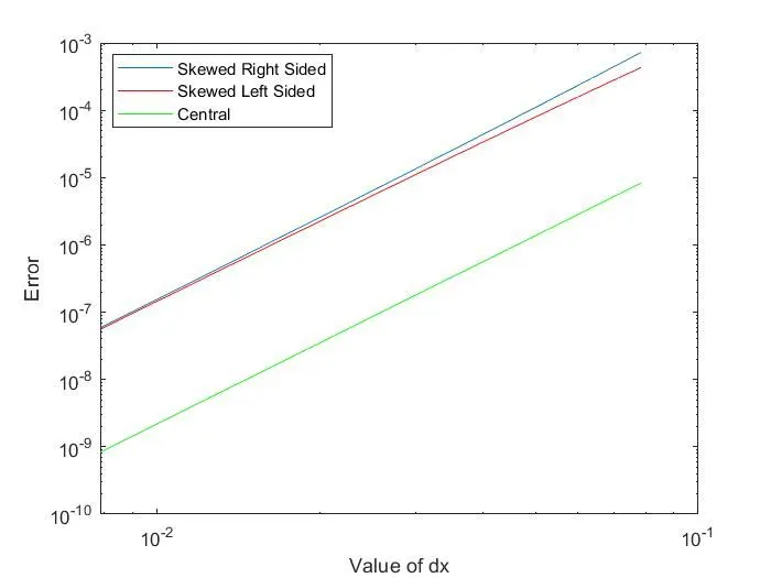
• As the error values are found, the comparison plot is made using the 'loglog' command with 'dx' along x-axis and 'Errors' along y-axis. (Note: As the variation between the errors of various schemes is drastic, this command is used to make a meaningful comparison).
• 'Hold on' command is used to stitch the multiple plots in the same graph.
• 'Legend' and 'label' are given to add meaning to the plot.

Output Explanation:

• Output Screen Shot:
  • 
    • Observations and Inference:
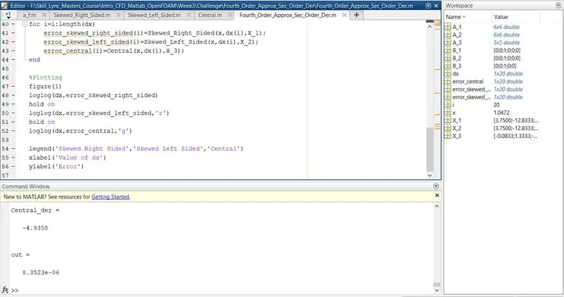
      • The workspace pane ascertains that there are 20 values for error associated with each type of scheme owing to 20 different values of dx.
      • Also, the Taylor table coefficients are displayed in the command window and in the workspace pane.
• Comparison Plot:
  • 
    • Observation and Inference:
      • Overall, the error value for the central difference scheme is the lowest for the range of dx taken.
      • The error value for both the skewed right-sided scheme and the skewed left-sided scheme are almost equal, but as the dx value increases the error value of left-sided scheme becomes slightly lower than that of the right-sided one.
      • For the taken range of dx, the error increases as the dx value increases, otherwise, the error decreases as the dx value decreases for all the schemes.

Significance of a skewed scheme over a central scheme:

• A skewed scheme is useful because, this scheme is capable of finding the first order approximation of a first order derivative for any given function.
  • Illustration:
    • For skewed scheme, the formula to find the number of nodes(n) is:
    • `n=p("order of derivative")+q("order of approx.")`
    • `=>"For this case: "n=1+1=bb2`
    • This means that, the reference node and a node before or after this node are taken to compute the derivative.
    • Whereas, for central or symmetric scheme, it is:
    • `n=p+q-1=>n=1+1-1=bb1`
    • As the derivative can't be found with a single node alone, for the node being the reference node, i.e., the point at which the derivative has to be found. It is not possible to find the first order approximation of first order derivative using the central scheme.
    • Therefore, the skewed scheme is useful in this way!
• Moreover, a skewed scheme is very useful in computing the values for one-sided flows, i.e.,
  • If the flow is from left to right, then skewed left-sided scheme is used; else if the flow is from right to left, skewed right-sided scheme is employed.
• While a skewed scheme is significant in this application; a central scheme is used in cases where diffusion or infusion takes place and the data from all directions are required to compute the values.

Result:

• Thus, the formula for the fourth order approximation of a second order derivative has been derived and coded using Matlab.
• Also, the code has been used to numerically compute the second derivative of a given analytical function; a comparison graph of the error associated(w.r.t., analytical derivative) plotted and the inferences derived.
• Finally, the question posted has been answered with a relevant example.