Week 3.5 - Deriving 4th order approximation of a 2nd order derivative using Taylor Table method

OBJECTIVE:

Deriving the fourth order schemes for the second order derivative using the "central differencing","skewed right","skewed left" schemes,with the taylor table method. To simplify the algebraic calculations and to find the co-efficients easily the taylor series expansion is used with the table format.

GIVEN FUNCTION :

> exp(x)*cos(x)

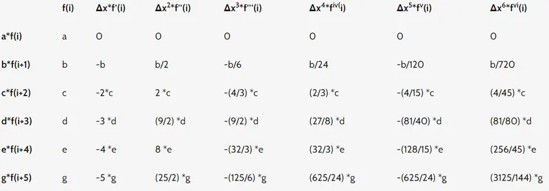
Taylor table for the fourth order approximations of second order derivative:

1. Central difference scheme:

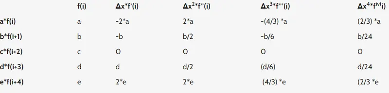
Considering four grid points except f(i), which will be leading to the fourth order scheme of second order derivative.

2. Skewed right scheme:

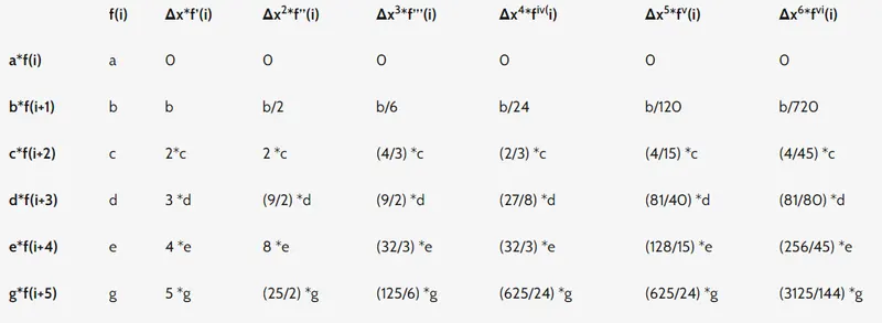
Skewed schemes are used in place of central difference schemes where at boundary conditions or layers the central difference schemes has no grid points and so skewed schemes will help to capture the accuracy.

3. Skewed left scheme:

FORMULA USED TO CALCULATE THE NUMBER OF TERMS:

N = [A+O-1]

here we are about to find the fourth order approximations,

hence

A = 4,

O = 2,

And so N = 4+2-1 = 5, hence we are using five terms for the calculation.

CODE:

clear all
close all
clc

x = pi/3;

dx = linspace(pi/4,pi/4000,50);

%given function = exp(x)*cos(x)
Analytical2nd_derivative = -2*exp(x)*sin(x);


for i = 1:length(dx)
    
    a(i) = exp(x-(5*dx(i)))*cos(x-(5*dx(i)));
    b(i) = exp(x-(4*dx(i)))*cos(x-(4*dx(i)));
    c(i) = exp(x-(3*dx(i)))*cos(x-(3*dx(i)));
    d(i) = exp(x-(2*dx(i)))*cos(x-(2*dx(i)));
    e(i) = exp(x-dx(i))*cos(x-dx(i));
    f(i) = exp(x)*cos(x);
    g(i) = exp(x+dx(i))*cos(x+dx(i));
    h(i) = exp(x+(2*dx(i)))*cos(x+(2*dx(i)));
    j(i) = exp(x+(3*dx(i)))*cos(x+(3*dx(i)));
    k(i) = exp(x+(4*dx(i)))*cos(x+(4*dx(i)));
    l(i) = exp(x+(5*dx(i)))*cos(x+(5*dx(i)));
   
    
     FDS(i) = forward_diff_scheme(g(i),f(i),dx(i));
     BDS(i) = backward_diff_scheme(e(i),f(i),dx(i));
     CDS(i) = central_diff_scheme(d(i),e(i),f(i),g(i),h(i),dx(i));
     SkdR(i) = skewedright_diff_scheme(f(i),g(i),h(i),j(i),k(i),l(i),dx(i));
     SkdL(i) = skewedleft_diff_scheme(f(i),e(i),d(i),c(i),b(i),a(i),dx(i));
      

  error_fds(i) = abs(FDS(i)-Analytical2nd_derivative);
  error_bds(i) = abs(BDS(i)-Analytical2nd_derivative);
  error_cds(i) = abs(CDS(i)-Analytical2nd_derivative);
  error_skdl(i) = abs(SkdL(i)-Analytical2nd_derivative);
  error_skdr(i) = abs(SkdR(i)-Analytical2nd_derivative);
end

% hold on
% loglog(dx,error_fds,'linewidth',1,'marker','.')
% hold on
% loglog(dx,error_bds,'linewidth',1,'marker','*')
%  hold on
 loglog(dx,error_cds,'linewidth',1,'marker','+')
hold on
loglog(dx,error_skdl,'linewidth',1,'marker','pentagram')
hold on
loglog(dx,error_skdr,'linewidth',1,'marker','hexagram')

xlabel('dx')
ylabel('error')
legend('Central differencing','skewed right','skewed left');
% axis([0 0.1 0 1]);

FUNCTION CODE FOR CENTRAL DIFFERENCE:

function [cds] = central_diff_scheme(a,b,c,d,e,f)

cds = (-a+16*b-30*c+16*d-e)/(12*f^2);

end

FUNCTION CODE FOR SKEWED RIGHT SCHEME:

function [skdr] = skewedright_diff_scheme(a,b,c,d,e,f,g)

skdr = ((45*a)-(154*b)+(214*c)-(156*d)+(61*e)-(10*f))/(12*(g^2));

end

FUNCTION CODE FOR SKEWED LEFT SCHEME:

function [skdl] = skewedleft_diff_scheme(a,b,c,d,e,f,g)

skdl = ((45*a)-(154*b)+(214*c)-(156*d)+(61*e)-(10*f))/(12*(g^2));

end

FUNCTION CODE FOR FORWARD DIFFERENCE SCHEME:

function [fds] = forward_diff_scheme(a,b,c)

fds = (a-b)/c;

end

FUNCTION CODE FOR BACKWARD DIFFERENCE SCHEME:

function [bds] = backward_diff_scheme(a,b,c)

bds = (b-a)/c;

end

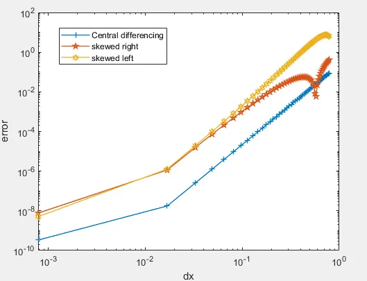
OUTPUT PLOT:

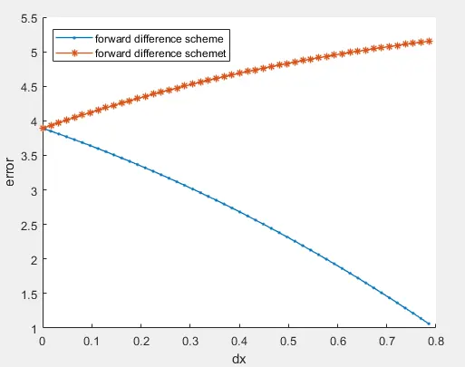
For FDS and BDS:

DISCUSSION:

The central difference scheme has the lower order of error comparing to the skewed schemes, and also the error is in increasing fashion for increased grid size.

Also the skewed schemes will be used in place of central difference schemes where at boundary layers there won't be a left/right grid points and so will have to choose some imaginary points and which is highly difficult.