Week 2 Railwheel and Track
AIM :
To Perform a Static Structural Analysis on the Rail Wheel & Track setup. All Should be done by Using ANSYS.
OBJECTIVES :
To Perform a Static Structural Analysis on a setup with 100 KN & 500 KN as a Bearing load.
To Solve the Total Deformation, Equivalent Von Mises Stress and Life cycle of the Wheel.
To Solve the Total Deformation of a setup by User defined Expression.
PROCEDURE FOR ACHIEVING THE OBJECTIVES :
I) CAD Model :
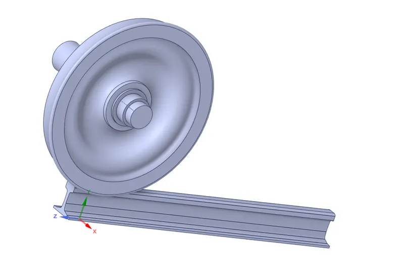
A Rail Wheel & Track Setup model is given from Design team. We have to import the model into Geometry section, inorder to verify the model before going to any process. Open a Space Claim or Design Modeller to which verify or edit the geometry based on our requirements. In this case, given model has been perfect, it's looks like as shown in the below image.
II) Material Assigning :
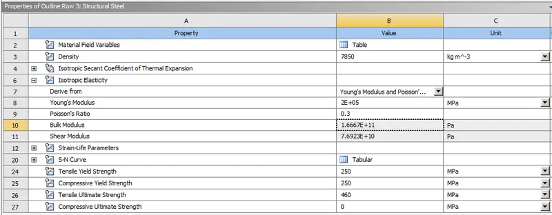
By Default, Structural Steel material is already added in the engineering data list and also we use same material for all components. Here below image, a Structural steel material properties are listed out.
Once Opened the mechanical model, we have to assigning the materials to the respective component.
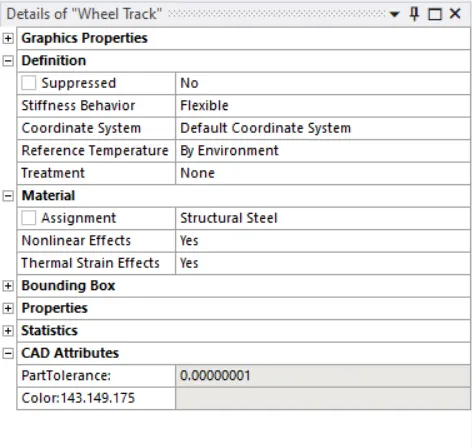
From below snap, I assigned the structural Steel as a material for Wheel Track. We use same material for remaining components which are Wheel & Axle.
III) Connections :
A Mechanical Model have inbulit algorithms for which predicting the contacts based on component touching to each other. Something, it might be helpful for us, in this case those contacts are useful.
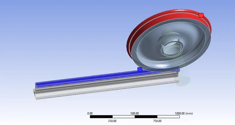
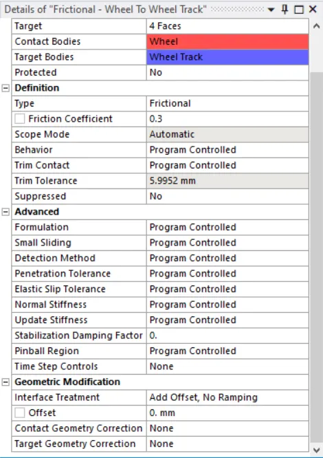
First Contacts is made between a Wheel to rail track like as shown in below image.
Type of Contact is Frictional with the frictional Coefficient of 0.3.
Keep Add Offset, No Ramping for Interface treatment.
Keep remaining options are as it is.
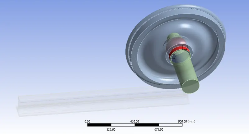
Second Contact is made between a Axle and Wheel like as shown in below image.
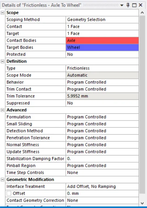
Type of contact is Frictionless. Because, it's a dead axle.
Keep Add Offset, No Ramping for Interface treatment.
Keep remaining options are as it is.
Joints :
Fixed Joint :
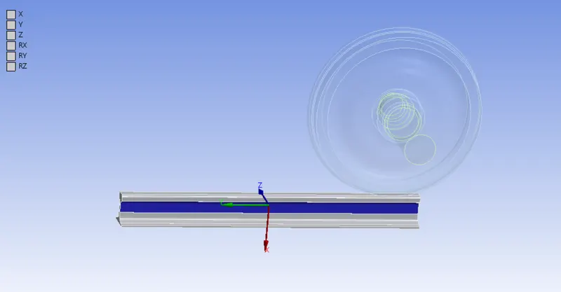
To Constraint the rail track to all possible degree of freedom by using Fixed Joint. Which means we fix the rail track into ground.
Displacement Joint :
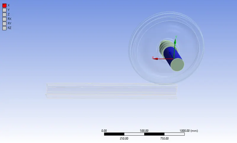
Select the Axle surface, constraint the all possible degree of freedom except translation on X direction. Which means axle can able to change the position on the x direction either positive or Negative according to the input.
Planer Joint :
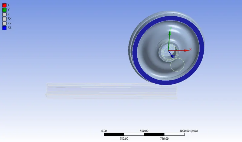
Select the face on the wheel, to constraint the wheel motion about translational Z direction, Rotational about X & Y axis except translation on X & Y and Rotational about Z axis by using Planer Joint.
IV) Meshing :
Basically, To divide the entire model into infinitesimal control volume, that frame work is called Meshing. This process is called Discritization. This FEM is widely used for solving partial differential equation in different physical field such as Structural problem, Heat transfer problem, Fluid flow problem, Electro magnetic Analysis & Acoustics Analysis.
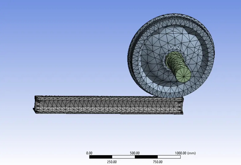
Element Size = 50 mm
Face Mesh Element Size = 35 mm
Element Type = Volumetric meshing with Tetrahedrons or Tetrahedrals element
No of Nodes = 13304
No of Elements = 6726
Reason for refine the face on the wheel & Track. Since, we interseted in looking at stress developed on near the face of the components. Inorder to get to capture the accurate results on that particular surface, we have to refine on it.
We keep "Program Controlled" for Element Order, so Ansys takes a second order elements, each Tetra elements have 10 nodes itself. By results, it take more time for solving as compared to First order elements & increasing storage space also. But, results has been more accurate as compared then first order discritization.
After done the meshing on the model, it has looks as shown in below image.
V) Analysis Settings :
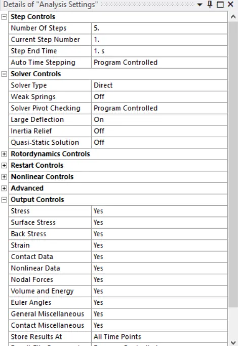
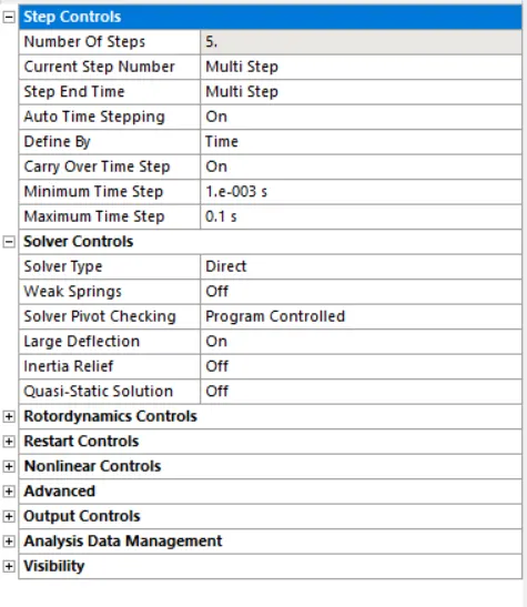
In this case, we can run the simulation upto 5 number of steps.
For Step 1,
Auto Time Stepping is "Program Controlled"
Solver Type is "Direct"
Large Deflection is "ON"
Switch to "Yes" for all parameter which are comes under the Output Controls.
For Step 2 to 5,
If we select the number of steps has morethan 1, a Current Step Number & Step End time are changed as "Multi Step"
Auto Time Stepping is "ON"
Define By "Time"
Carry Over Time Step is "On"
Minimum Time Step is "0.001 sec "
Maximum Time Step is " 0.1 sec "
Solver Type is "Direct"
Large Deflection is "ON"
Keep remaining options are as it is.
Boundary Conditions :
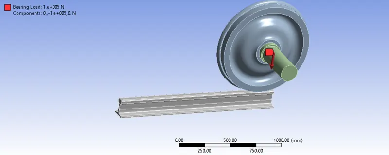
Bearing Load :
Usually, a train weight is acting on axle first and then it passess the same load to be applied on wheel as well. In this case, we applied an 100 & 500 KN as a bearing Load at downwards direction on the inner face of the wheel.
A same bearing load has been applied on the wheel at each steps.
Displacement Joint :
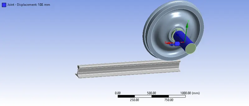
Provide the displacement at which on X direction from 0 mm to 500 mm with the interval 100 mm or 5 Steps.
Since, wheel is moving on positive in x direction, So we provide the distance value as positive numbers.
RESULTS :
Total Deformation :
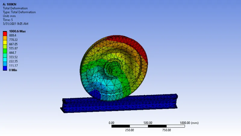
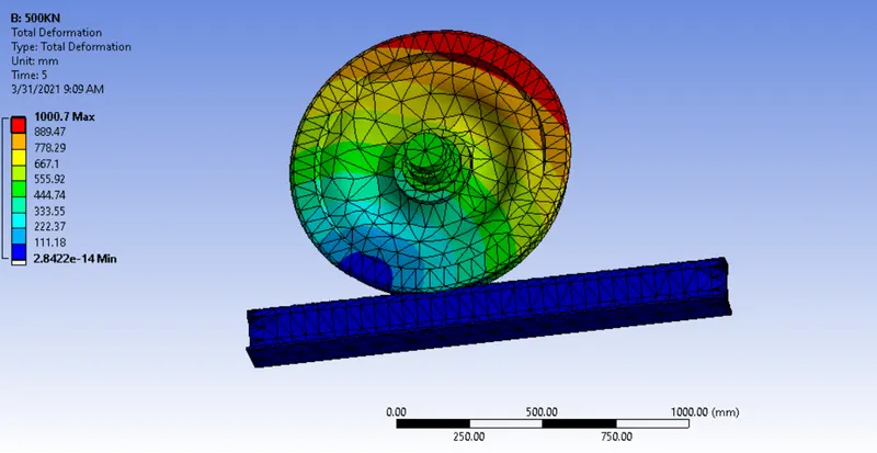
Total Deformation is same for both cases, a maximum deformation are generated at wheel while rotating.
Total Deformation for 100 KN :
Total Deformation for 500 KN :
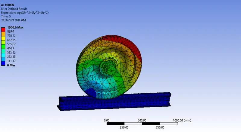
Total Deformation solving by User Defined Expression :
Total Deformation = `sqrt(Ux^2 + Uy^2 +Uz^2)`
By using this total deformation expression, we can solve the total deformation of the entire model, which is same as inbulit Result by ANSYS.
Equivalent Von Mises Stress :
If any rotating machine parts, we have to apply a load based on number of cycle which we want. A Life of Cycle has varying respect to applied load on the component.
As Stress strain curve point of view, a maximum stress shouldn't be exceed the yield stress of the material. If exceeding, a material will lead to fail.
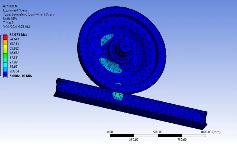
Equivalent Von Mises Stress for 100 KN :
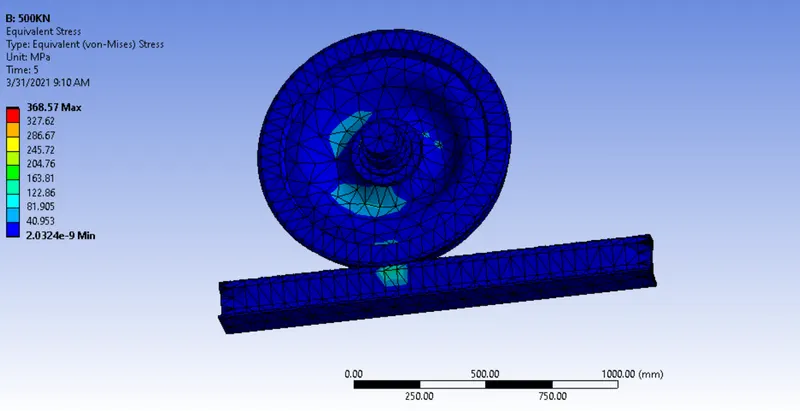
Equivalent Von Mises Stress for 200 KN:
Life Cycle of the Components :
Life cycles are calculated only for rotating parts or fluctuating stress developed on the component. By using SN Curve, we can calculate the Number of cycle with respect to corresponding stress.
For Case 1, a maximum stress generated value is around 84 Mpa, corresponding Number of cycles is 10e5. Which is High cycle in the SN Curve
For Case 2, a maximum stress generated value is around 370 Mpa, a corresponding number of cycles is 3482. Which is Low cycle in the SN Curve.
CONCLUSION :
| Bearing Load in N | Equivalent Von Mises Stress in Mpa | Total Deformation in mm | Life of the component in cycles |
| 100 KN | 83.975 | 1000.6 | 1000000 |
| 500 KN | 368.57 | 1000.7 | 3482 |
I perfer 100 KN load, because number of cycles are high and low stress developed in the component.