Week 2 Railwheel and Track
Challenge Task:
Case 1: Multiply the bearing load by 5 times and compare the results with the load of 100000 N. Compare the Total Deformation, Equivalent stress, and life under both the loads
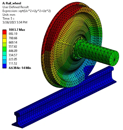
Case 2: Implement a User-defined result and calculate the Total Deformation from this result and check if it is the same as that obtained by the inbuilt result by ANSYS for a load of 100000 N.
Objective:
To perform Static Structural analysis of Rail Wheel and Track using ANSYS Workbench.
Geometry:
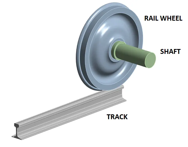
Shown below is the 3D Geometry of the Rail Wheel with Track, the Shaft is also attached to Rail Wheel.
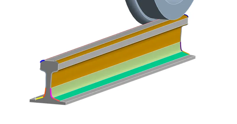
Note: In Mechanical Interface used virtual topology to fix the issue with small faces present in the geometry. By fixing this we could decrease the mesh node count and therefore save computational time.
Material Properties:
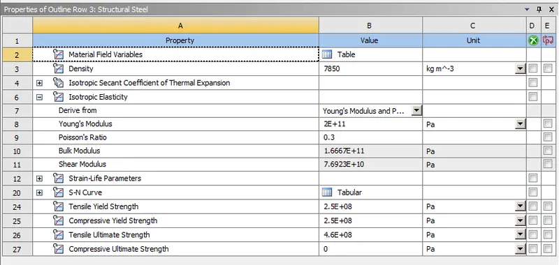
We have taken Structural Steel Material into consideration in this analysis.
Mesh Criterion:
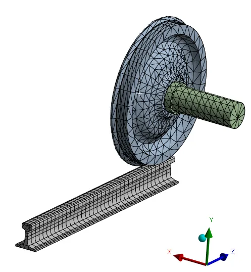
Meshed the component with the Automatic method and an element size of 50mm is deployed over the body and considered an element size of 35mm at the contact region faces. Also for capturing the circular features in the geometry used the Face meshing option.
Boundary Conditions:
- Two Contacts were made, One is Wheel to Track (Friction Co-efficient=0.3) and another is Shaft to Wheel (Friction Less).
- 3 Types of joints are considered one Track is fixed, in second Shaft is kept in translation, and in third wheel face is given planner joint on one of its faces.
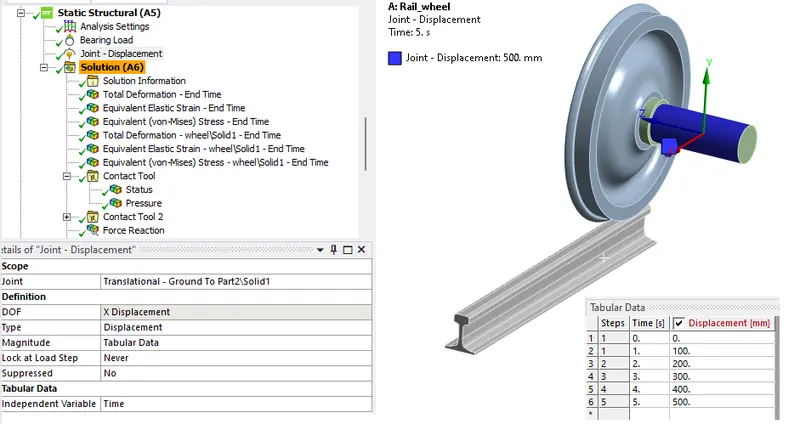
- Joint Displacement: Define the joint load for the shaft as a translation joint. so click on the static structural and select joint load, change the type as displacement and with a magnitude of 0, 100, 200, 300, 400, 500.
- Bearing Load: Now hide the shaft and select the inner surface of the hole and select the bearing load, define it by component, and add the value y = -1e5, which is termed Case-1
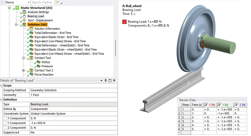
- Follow all the steps as similar for case-1, but just change the value Bearing load to y = -5e5 for the comparison study.
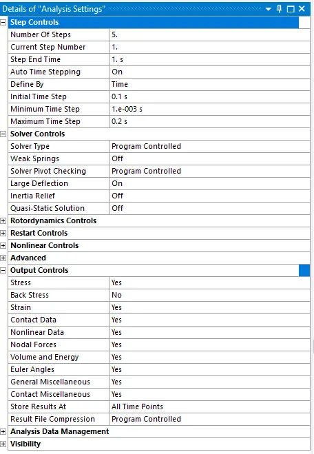
Analysis Settings:
No of Step = 5
Initial Time step = 0.1
Minimum Time step = 0.001
Maximum Time step = 0.2
Large Deformation as ON
Results and Conclusion:
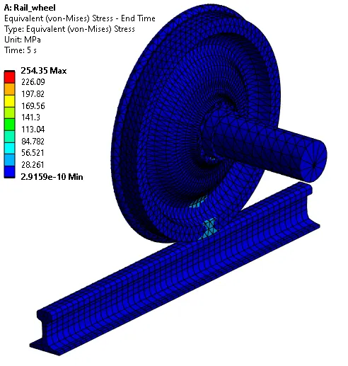
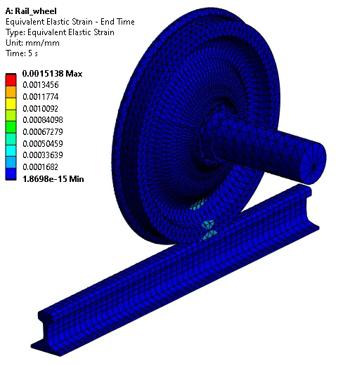
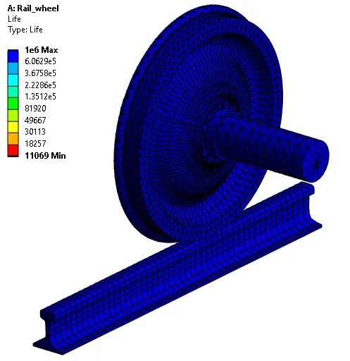
Simulation results for case-1 with different loads are as shown below.
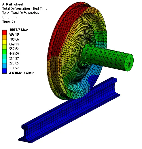
Case-1 with a Bearing load of 100000N.
Total Deformation:
Equivalent Stress:
Equivalent Strain:
Fatigue Life:
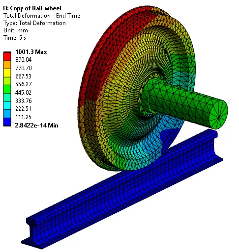
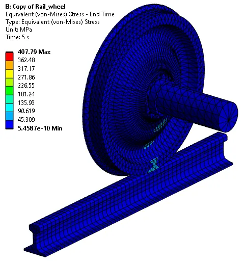
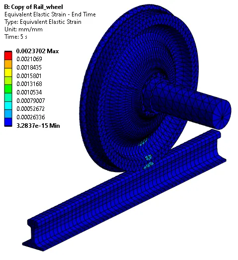
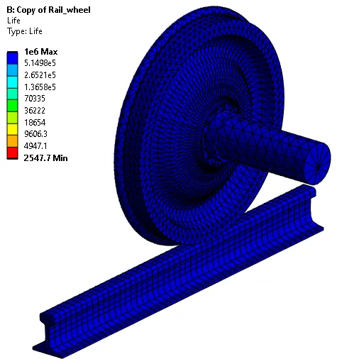
Case-1 with a Bearing load of 500000N.
Total Deformation:
Equivalent Stress:
Equivalent Strain:
Fatigue Life:
Case-2 Total Deformation of User-defined result and inbuilt result for a load of 100000N.
To find Total Deformation under User-defined result, we have input an expression sqrt(Ux^2+Uy^2+Uz^2)
User-defined results for Total Deformation:
In-built result for Total Deformation:
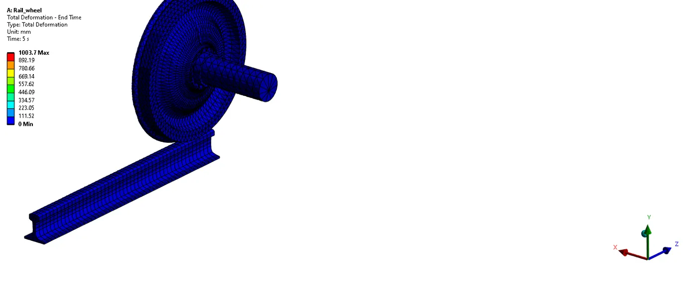
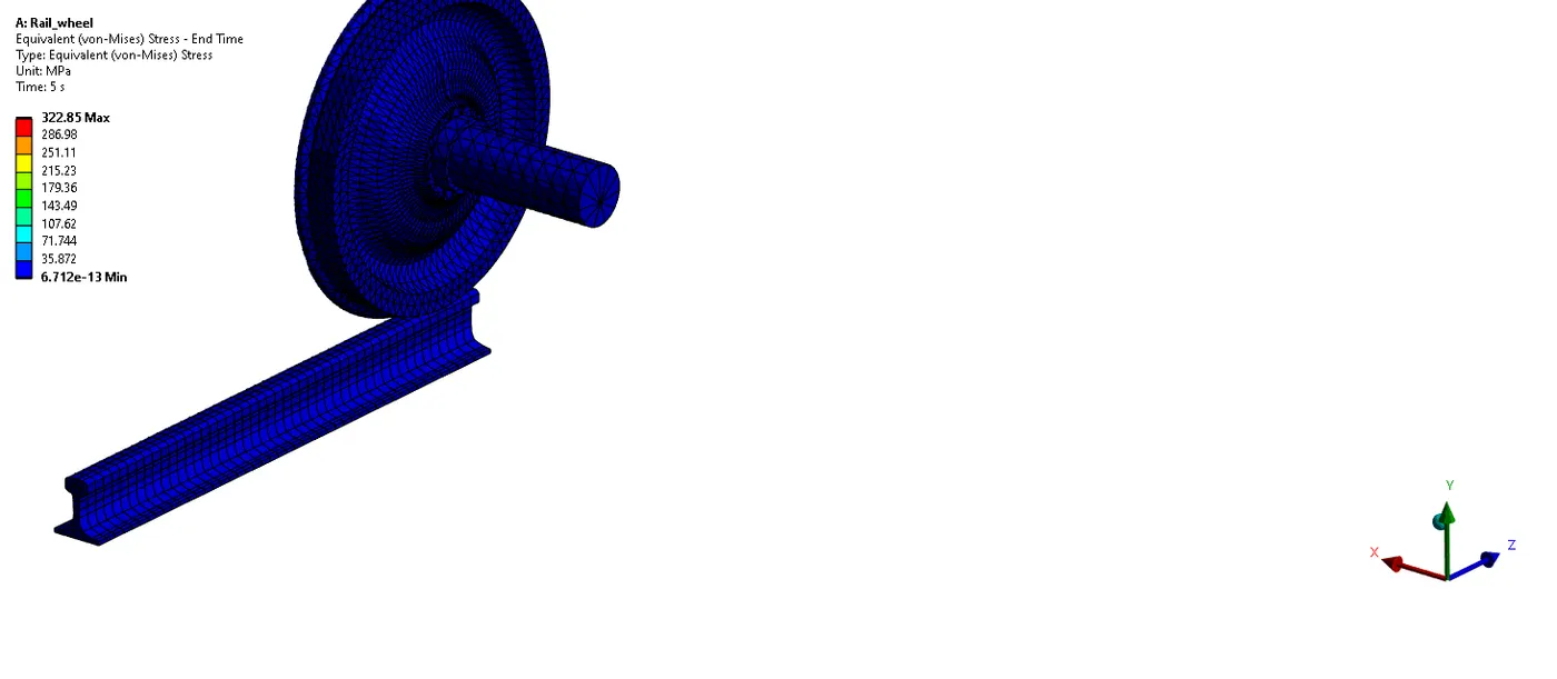
| SL No. | LOAD (N) | EQU: STRESS (MPa) | EQU: STRAIN (mm/mm) | TOTAL DEFORMATION (mm) | Max FATIGUE | Min FATIGUE |
| 1 | 100000 | 254.35 | 1.51E-03 | 1003.7 | 1E+06 | 11069 |
| 2 | 500000 | 407.79 | 2.37E-03 | 1001.3 | 1E+06 | 2548 |
Simulation
Total Deformation:
Equivalent Stress:
CONCLUSION:
Case 1: From the table, we can say that the stress is Maximum for a 500000N Load which is 407.79, and Minimum for 100000N Load which is 254.35. The Total deformation remains nearly the same in both cases. The Fatigue life for the higher load of 500000N has a low life of 2548 cycles compared to the 100000N load.
Case 2: The user-defined result for Total Deformation and the Inbuild result for Total Deformation is the same.
Link for Accessing the Workbench file and Simulation data: https://drive.google.com/drive/folders/1jLcB2qgFZ7VfX0ASmfQcI3kuda0k9clT?usp=share_link