Week 2 Railwheel and Track

AIM: - PERFORM A STATIC STRUCTURAL ANALYSIS ON THE RAIL WHEEL AND TRACK SETUP TO CALCULATE TOTAL DFEFORMATION, EQUIVALENT STRESS, AND THE LIFE FOR:

CASE 1: CHANGE THE BEARING LOAD TO 500 kN AND COMPARE THE RESULTS FOR THE TWO BEARING LOADS.

CASE 2: IMPLEMENT A USER-DEFINED RESULT TO CALCULATE TOTAL DEFORMATION AND COMPARE ITS OUTPUT WITH THE IN-BUILT RESULT FOR THE BEARING LOAD OF 100 kN.

Objectives:

Performing static structural analysis on the Rail Wheel and Track setup for two different bearing loads:

1. Bearing Load = 100 kN.
2. Bearing Load = 500 kN.

Calculate the Total Deformation, Equivalent Stress, and Life of the setup for both cases and compare.

Implement a User-Defined Result to calculate the Deformation and check if it is the same as the In-built result.

Rail Wheel and Track setup consist of:

1. Rail Wheel

2. Track

A Track is a permanent track line set up to allow the Rail Wheel to Roll over it. These are parallel lines acting as the foundation pathway or the guideways for the Rail Wheels. The tracks are generally made of Steel or Iron.

The two parallel railway track lines are supported from beneath with the help of Wooden Cross Ties, placed perpendicular to the tracks and maintaining a uniform gap between the two cross ties. In this gap crushed stones (Ballast) are filled to support the ties. Now, the Cross Ties used are made of Concrete.

Rail Wheels are the components that bear all the load of the carriage and perform the rolling motion over the tracks. The rail wheels are the most crucial component of a rail as even a minute deformity in the wheel may lead to catastrophic damage to life and property. This holds true for the track also.

Hence, both the components must be structurally fit for the operation at all times.

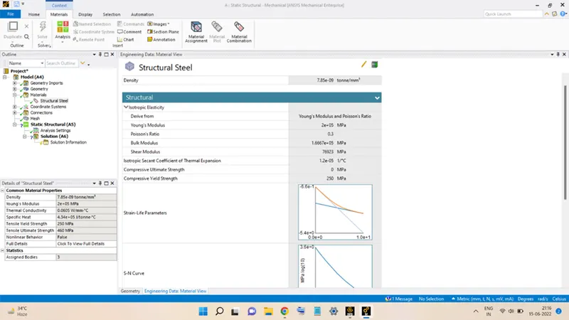
To begin with, the analysis, select the Static Structural Analysis from the Analysis Systems in the Ansys Workbench. Next, the material to be used is the Structural Steel present in the project as the default material.

Then, right-click on Geometry and click on Import to add the geometry into the project environment.

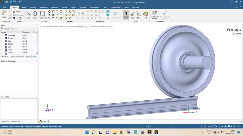
The imported geometry in SpaceClaim will look like this:

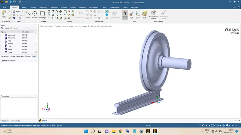
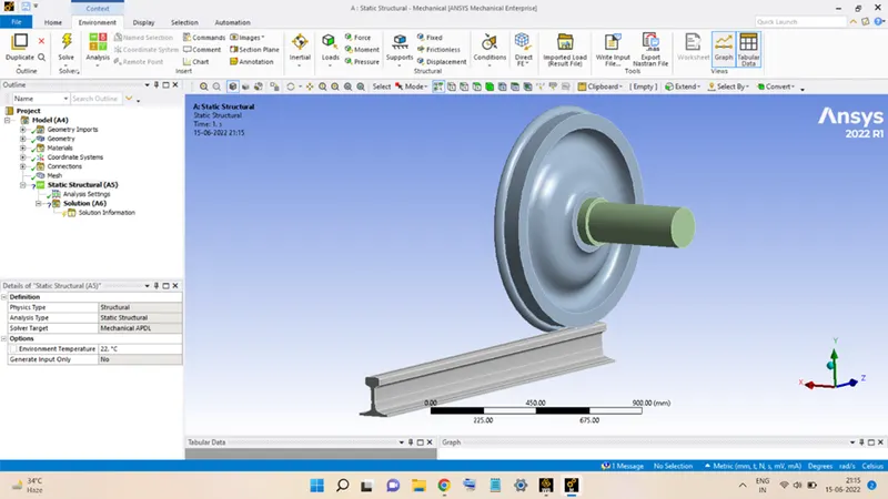
Now, double-click on Model to launch the Mechanical Module and load the geometry into the module. The geometry, in the Mechanical module, will look like this:

The properties of Structural Steel are shown below:

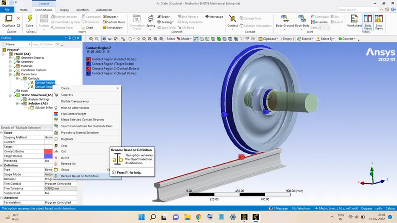
Next step is to apply the Contact conditions to the geometry. To do so, expand the Contacts option present in the Connections menu. First select both the Contact Regions then right-click and select Rename Based on Definition, as shown below:

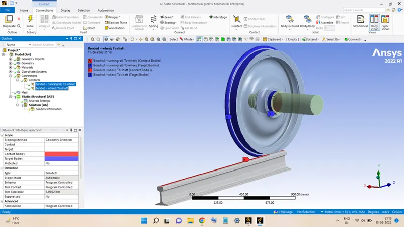
The names of the Contact Region will change, as shown below:

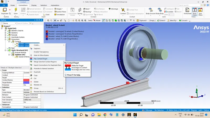
After this, again select both the contact regions and right-click and select Flip Contact/Target. It will flip the contact and target bodies in the geometry. As shown below:

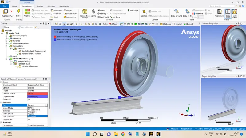
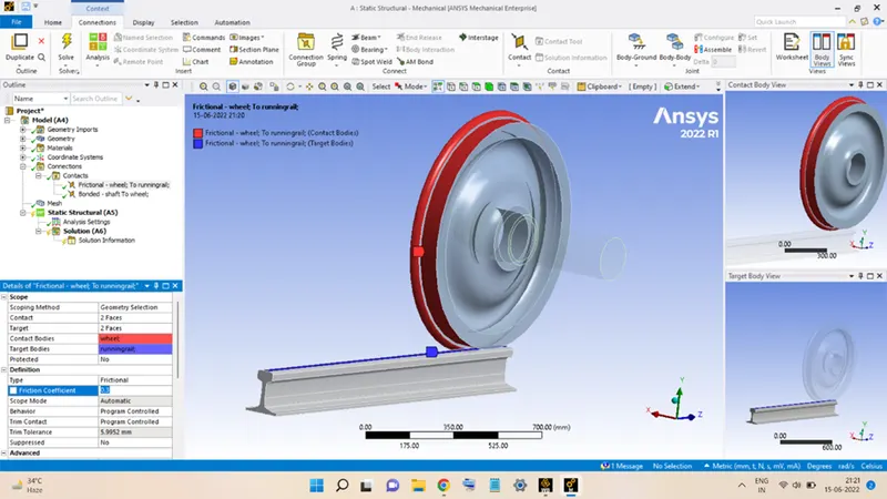
Select the contact between Wheel and Track, fix the Type as Frictional and enter the magnitude of Friction Coefficient as 0.3, as shown below:

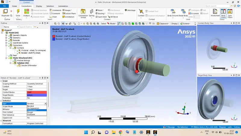
Now, select the contact between Wheel and Shaft and assign the Type as Frictionless.

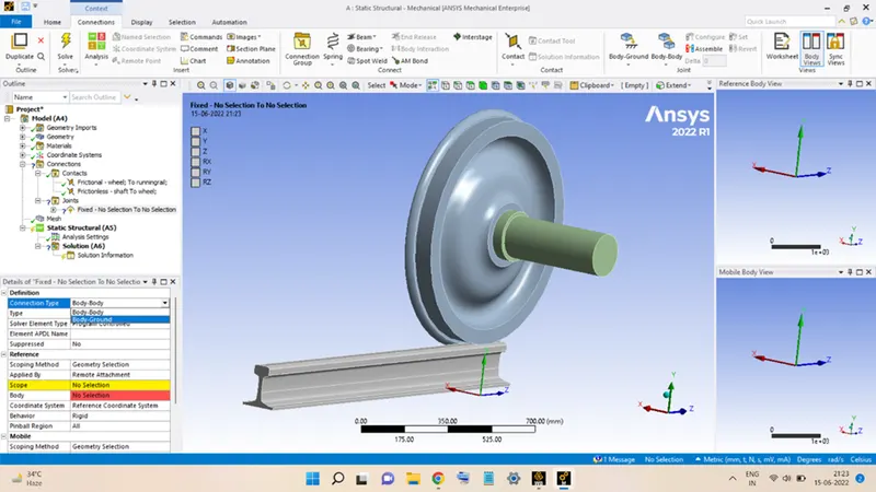
The next step is to assign the Joints in the geometry. To do so, right-click on Connections, go to Insert, and select Joint.

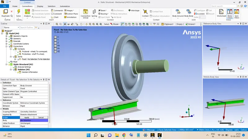
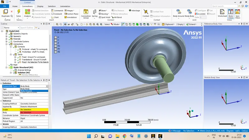
In the Definition section, select Body-Ground for the Connection Type.

Select Fixed for Type.

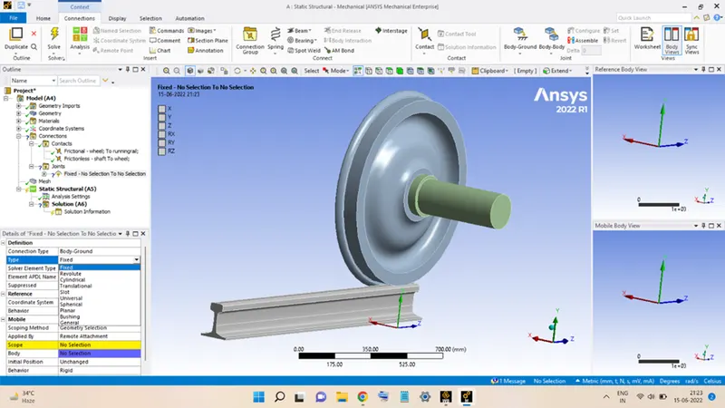
Then, select the two faces of the Track, as shown in the figure below, and hit Apply.

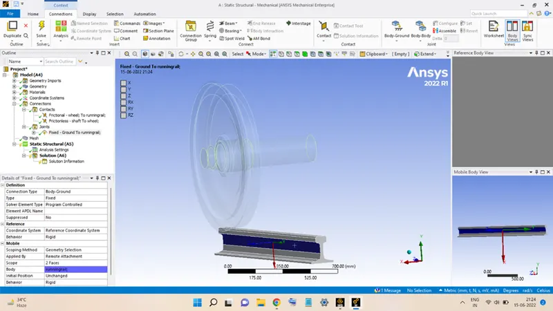
The Track will be fixed to the ground as shown below:

Now add a joint for the Shaft, such that the shaft can perform the translational motion along the Track. To do so, add another joint, then assign the Connection Type as Body-Ground, then select the Type as Translational.

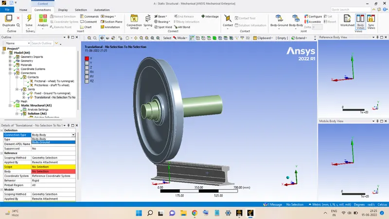
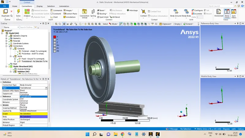
Then, select the Shaft surface and hit Apply.

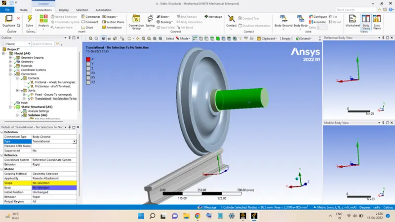
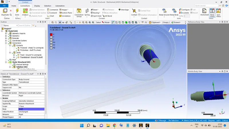
But, as seen from the figure, the shaft motion will occur in X-Axis (in red), which is not aligned along the Track's longitudinal direction.

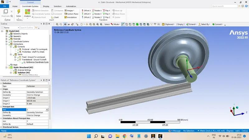
To align the X-Axis of the shaft, expand the Shaft and Ground joint, and select Reference Coordinate System. Go to the Principal Axis section and change the Axis to Z.

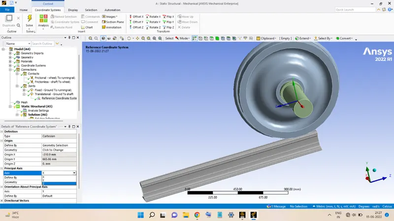
Now, the X-Axis of the shaft is aligned with the longitudinal direction of the Track.

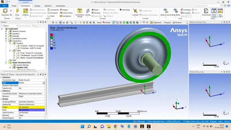
Now, add a planar joint in the geometry for the Wheel to remain in the current plane. To do so, add another joint, then select the Connection Type as Body-Ground and the Type as Planar Joint.

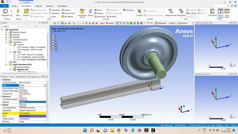
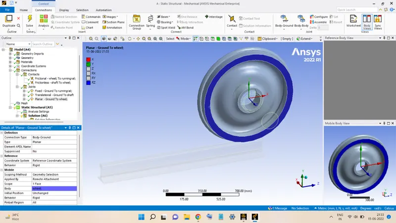
Then select the surface of the Wheel as shown in figure below and then hit Apply to add this joint in the geometry.

The next step is to mesh the geometry. This is done by clicking on the Mesh option and setting the Element Size equal to 50 mm and then right-click and hit Generate Mesh. The mesh generated will look like this:

Next is to add finer mesh to few areas of interest. To do this, right-click on Mesh, go to Insert select Sizing.

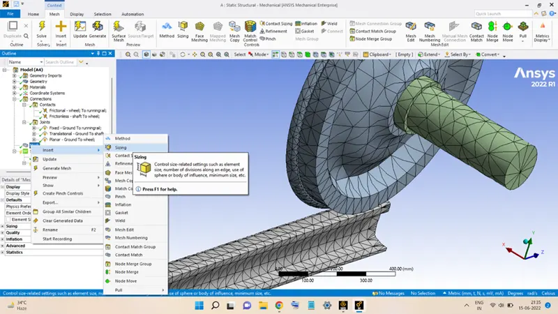
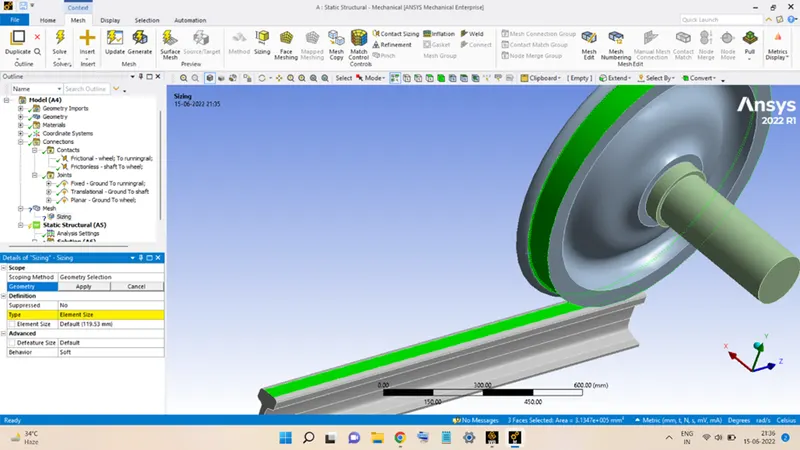
Select two surfaces on the Wheel and one surface on the Track and click on Apply, as shown in the figure below:

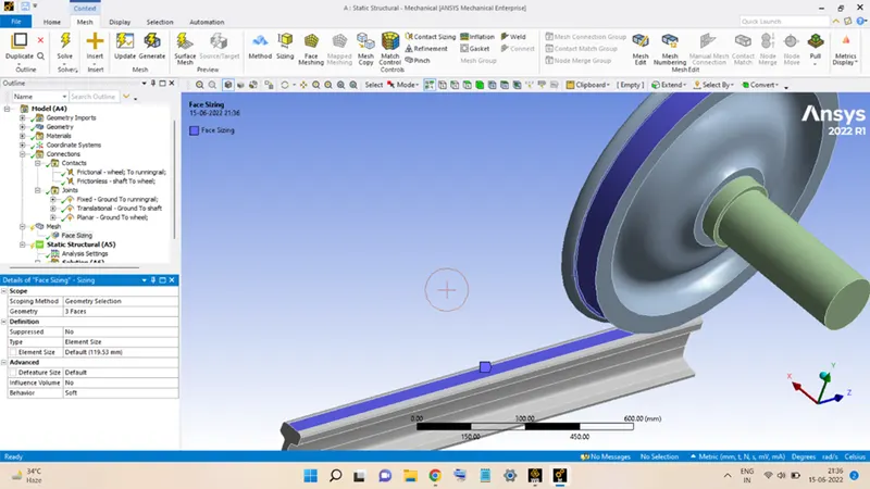
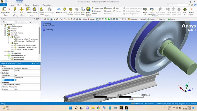
Finally, set the Element Size equal to 35 mm then right-click and select Generate Mesh.

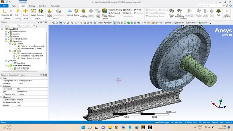
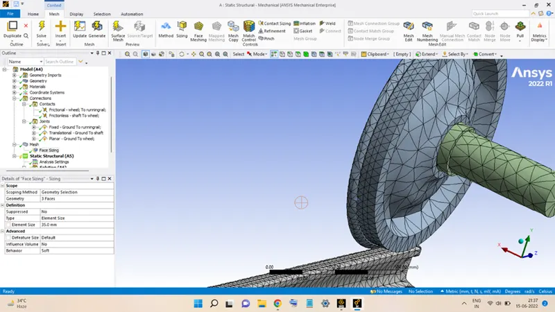
The next step is to assign the Analysis Settings to the geometry. To do so, click on Analysis Settings and then:

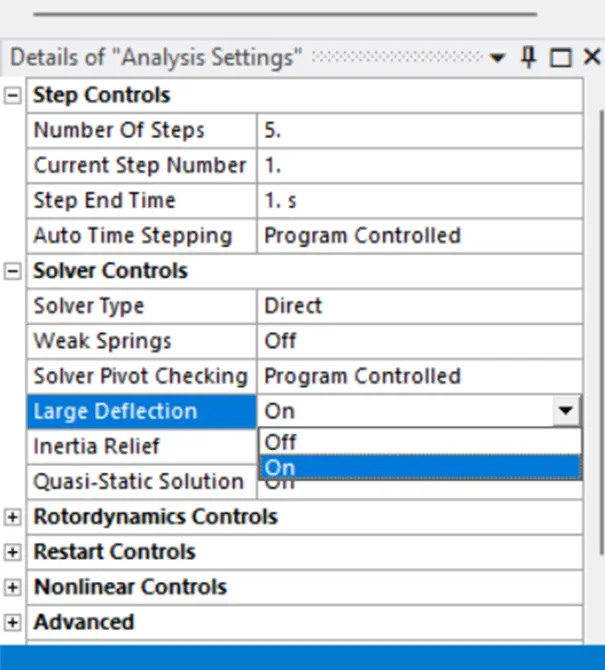
Set the Number of Steps equal to 5.

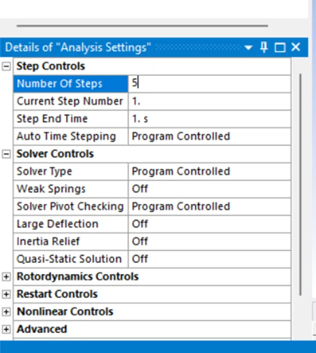
Keep the Current Step Number as 1 and Auto Time Stepping as Program Controlled and Solver Type taken will be Direct.

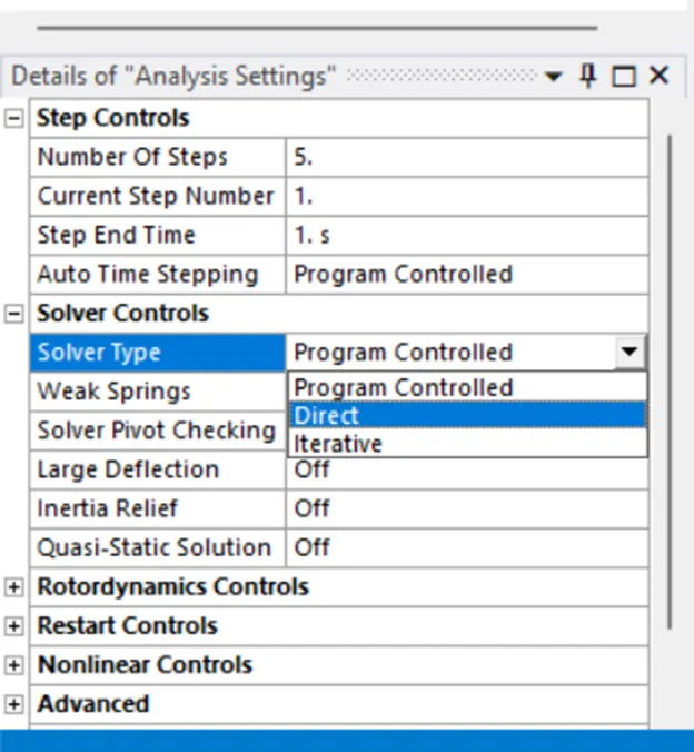
Large Deflection is turned ON.

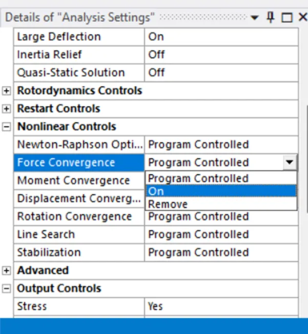
Force Convergence is turned ON.

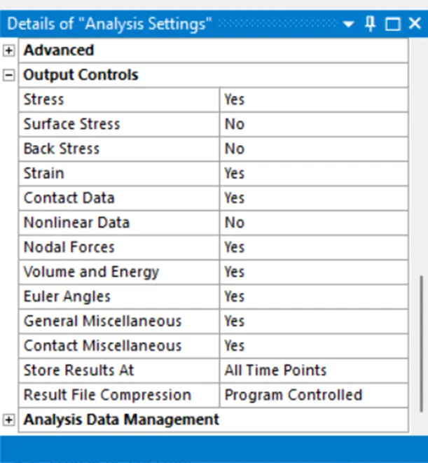
In Output Controls set the quantities to YES, as shown in the figure below:

Now for the remaining Time Steps, select all the remaining Time Steps, and Auto Time Stepping is turned ON and Defined By is changed to Time, and Carry Over Time Step is turned ON.

Set the Minimum Time Step as 0.001 sec and Maximum Time Step as 0.1 sec. And the rest settings are the same as those done for the First Time Step.

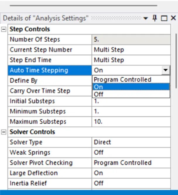
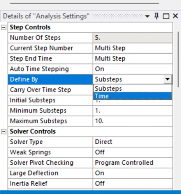
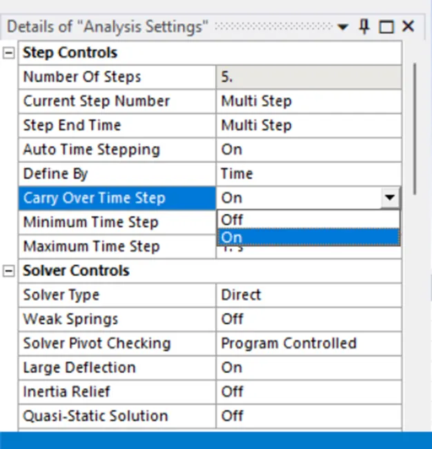
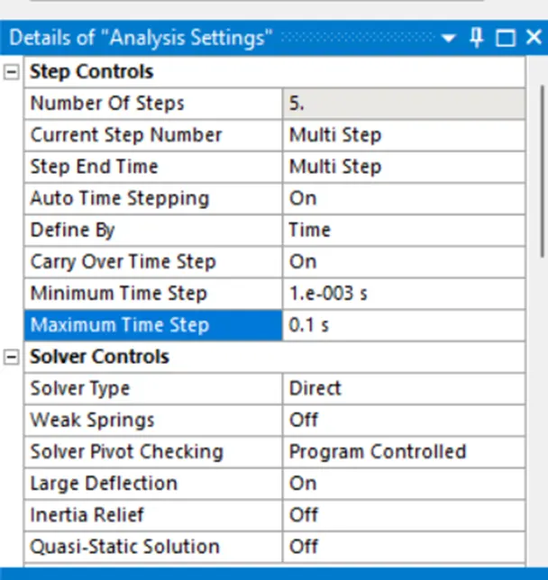
With this, the Analysis Settings are successfully assigned to the geometry.

Now the next thing to do is to assign the Joint Loads to the geometry.

To do so, right-click on Analysis Settings and go to Insert and Select Joint Load.

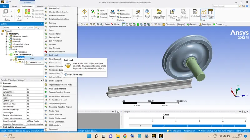
First, select the Translational – Ground To Shaft joint. Take the Type as Displacement, Magnitude is set as Tabular.

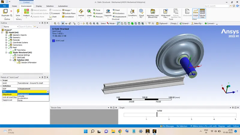
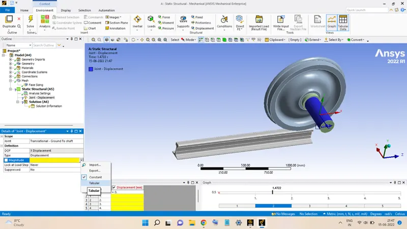
Then, add the values of the displacements for each Time Step as shown in the figure below:

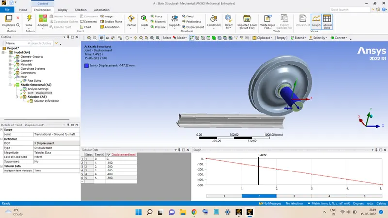
Next is to add the Bearing Load on the Wheel. To do so, first, the Shaft is hidden from the view by selecting the Shaft surface then right-click and select Hide Body.

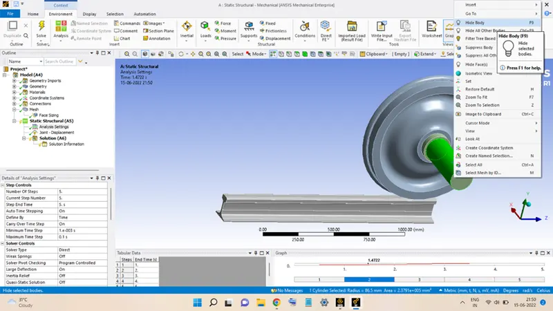
Next, select the inner surface of the Wheel and click on Loads, and select Bearing Load.

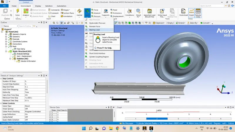
Magnitude is set to Components, and the load of magnitude 100 kN is applied on the surface in the negative Y-direction.

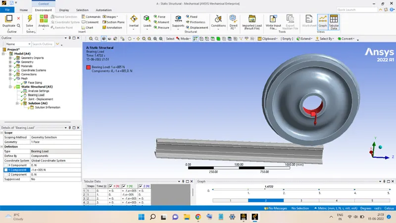
Then right-click and select Show all bodies to show the shaft also.

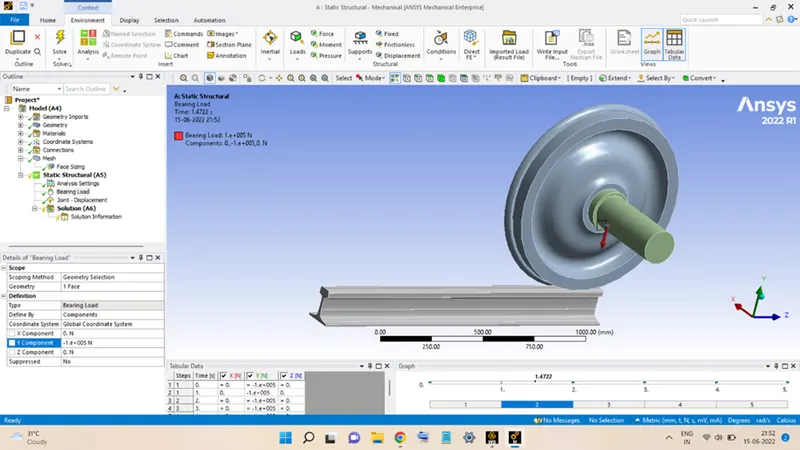
With this, the geometry is successfully assigned with the analysis settings as well as the loads.

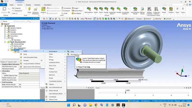
Now, the appropriate result quantities are to be added into the analysis, this is done by right-clicking on Solution going to Insert, and selecting the different quantities, which are as follows:

Total Deformation:

Equivalent Stress (for all bodies):

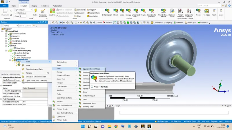
Equivalent Strain (for all bodies):

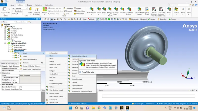
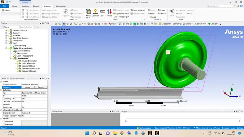
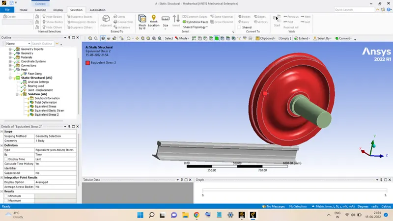
Equivalent Stress 2 (for Wheel only):

This is done by selecting the Wheel body and then clicking on the Geometry option and hitting Apply.

Equivalent Strain 2 (for Wheel only):

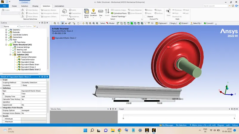
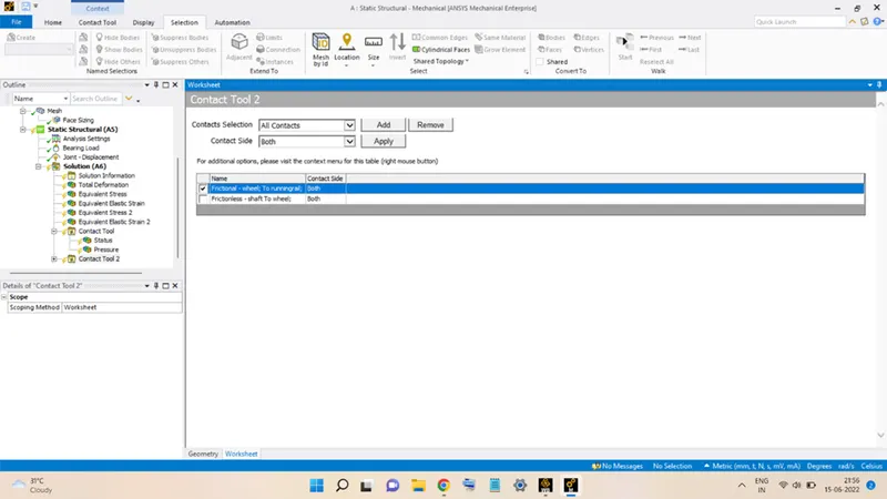
Contact Tool:

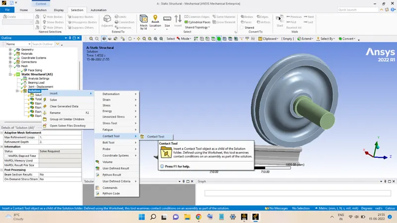
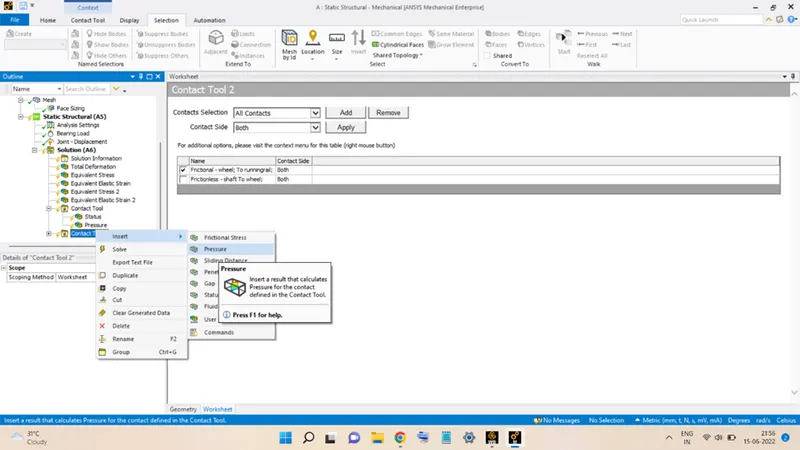
Select the Shaft to Wheel Contact and then add Pressure in the Contact Tool by right-clicking on it, then going to Insert and selecting Pressure.

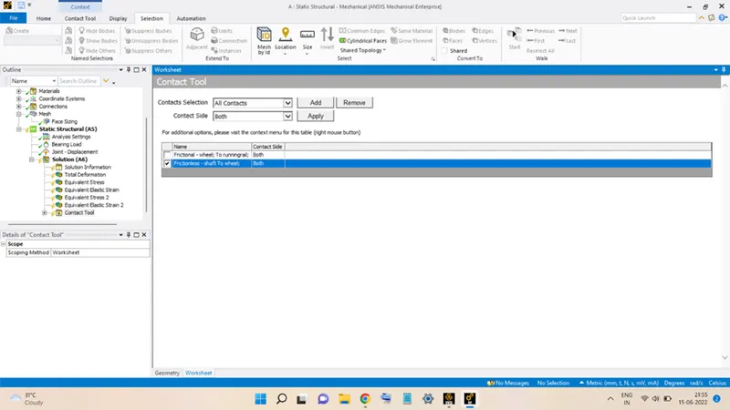
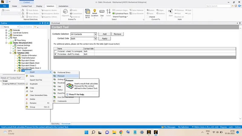
Do the same for the contact between Track and the Wheel, as shown below:

Probe:

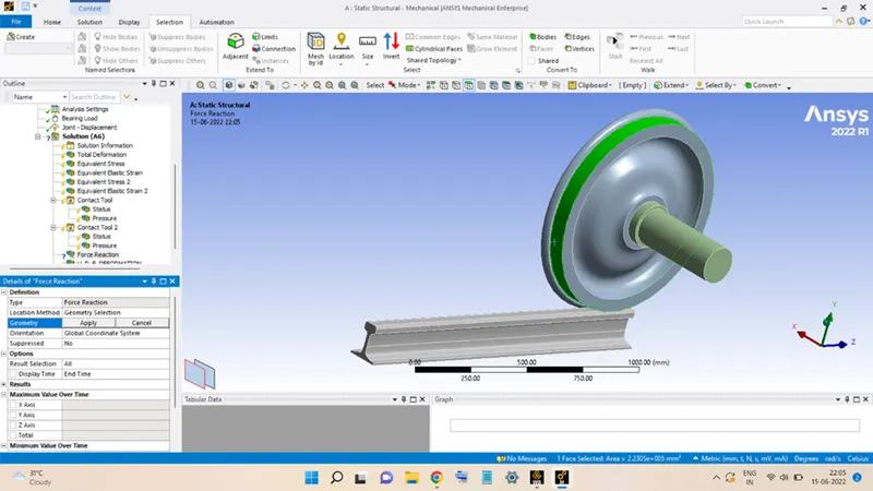
The probe is added by right-clicking on Solution then going to Insert and selecting Probe. In the Definition section, set the Type as Force Reaction and set the Location Method to Geometry Selection. Then select the surface of the Wheel and click Apply.

User-defined Result: Deformation

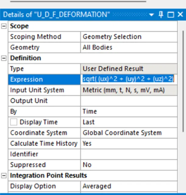
For the current problem, a User-defined Result is also required to be added to the analysis. The Output quantity is the Total Deformation experienced.

Mathematically, the expression for the total deformation is given as:

U_T = [ (U_x)² + (U_y)² + (U_z)² ]^0.5

Where,

U_T = Total deformation.

U_x = Deformation along X-Axis.

U_y = Deformation along Y-Axis.

U_z = Deformation along Z-Axis.

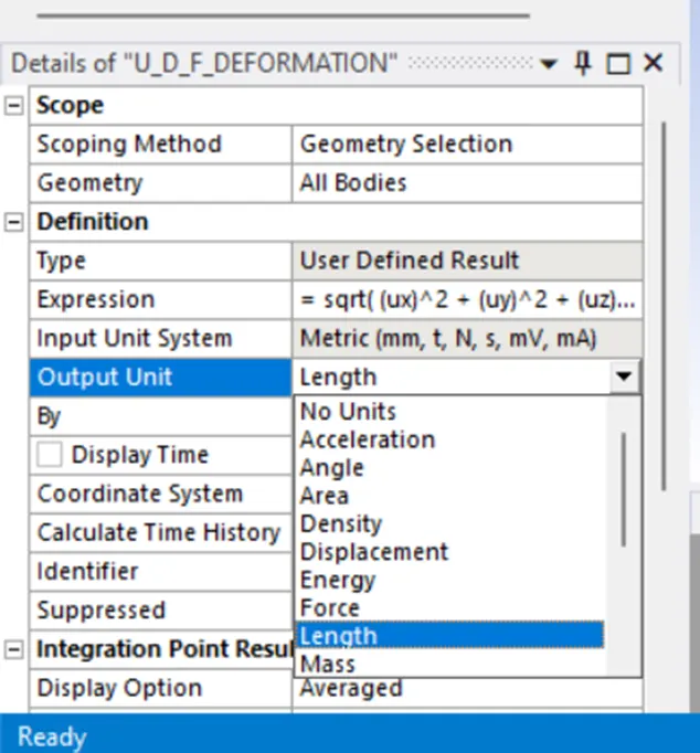
To add this as a User-Defined Result, right-click on Solution and go to Insert, and select User-Defined Result. Then, click on Expression and then feed in the expression of the result into the box Set the Output Unit as Length, as shown in the figure below:

With this, the analysis for CASE-1 is ready, click on Solve to begin the analysis.

The figure below shows the first Force Convergence.

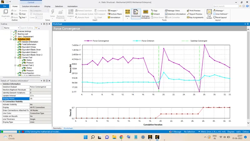
After the analysis is complete, the useful results are saved and then the Bearing Load is changed to 500 kN. For this case, the User-Defined Result (Total Deformation) is not included in the analysis. Then, the analysis is executed.

The results for both cases are mentioned below.

RESULTS

CASE 1: Bearing Load of 100 kN

Equivalent Stress:

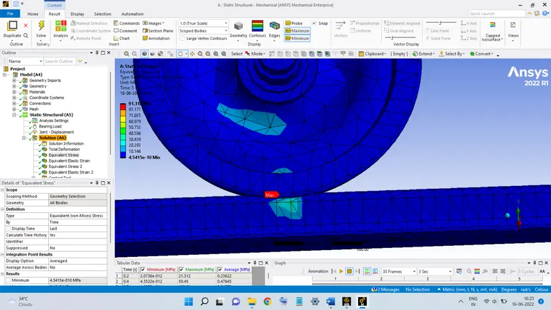
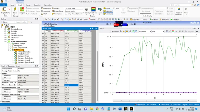
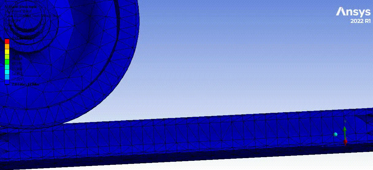
The maximum stress developed in the configuration is seen to be 155.96 MPa.

Equivalent Strain:

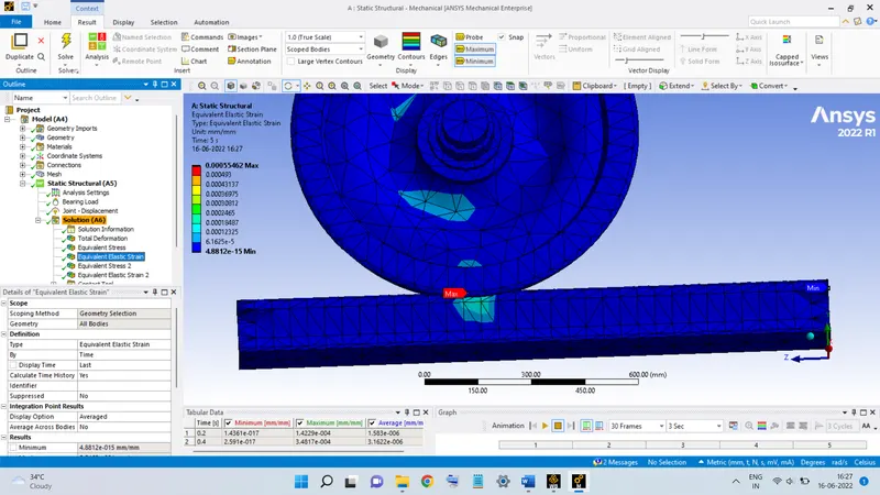
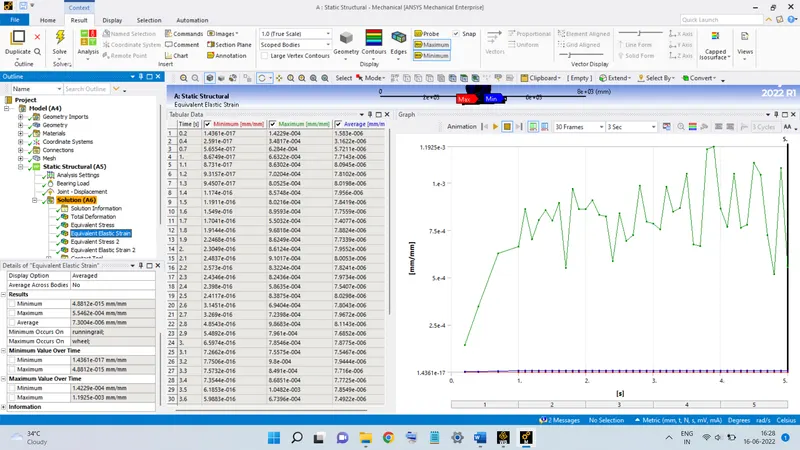
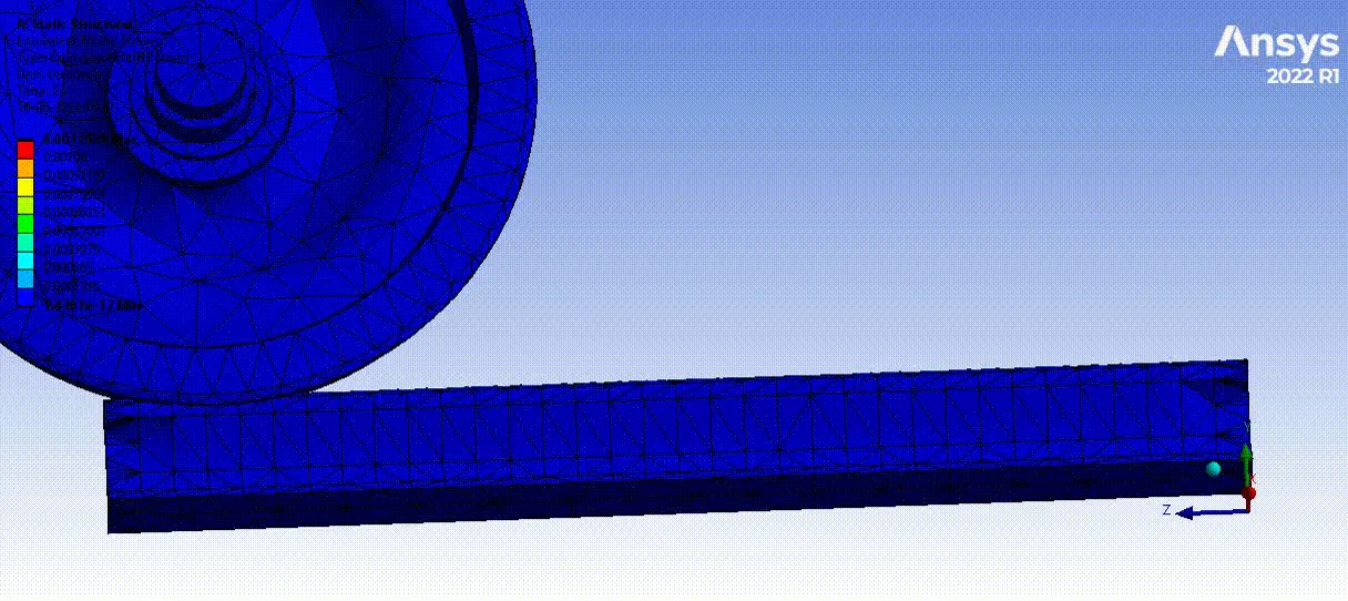
The maximum value of the strain is 1.1925 x 10^-3.

Stress in Wheel:

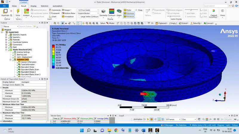
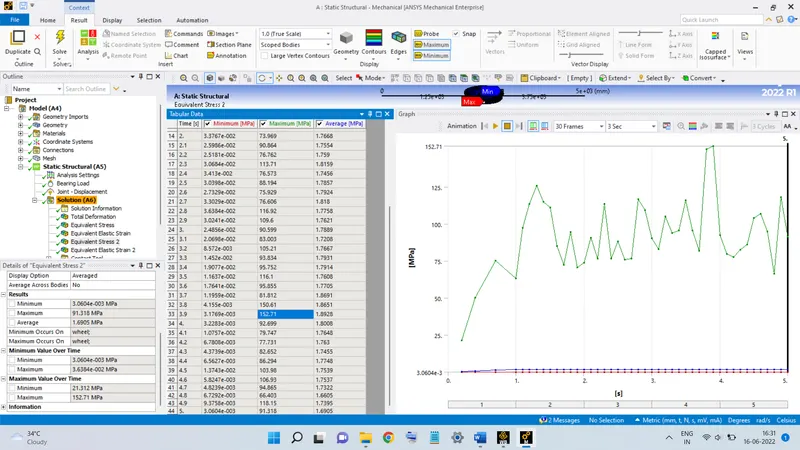
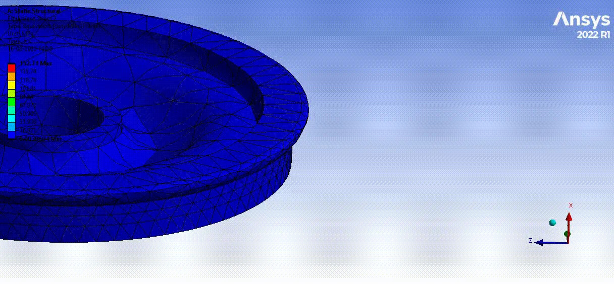
The maximum stress developed in the wheel alone is seen to be 152.71 MPa.

Strain in Wheel:

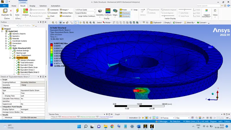
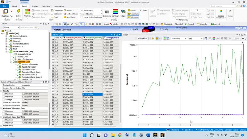
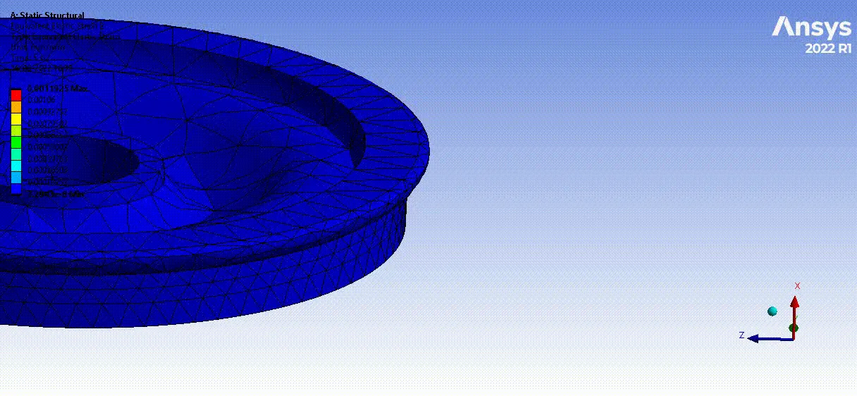
The maximum value of the strain in the wheel alone is 1.1925 x 10^-3.

Total Deformation:

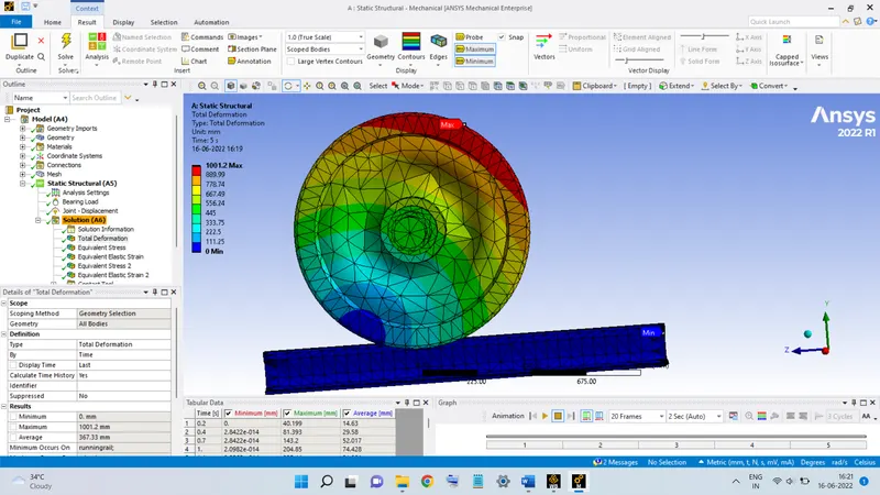
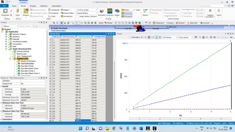
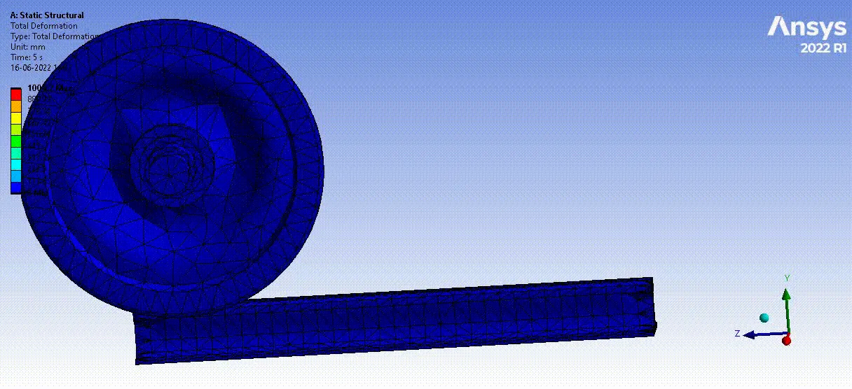
From the above figures, the maximum deformation is equal to 1001.2 mm.

Pressure between Wheel and Track:

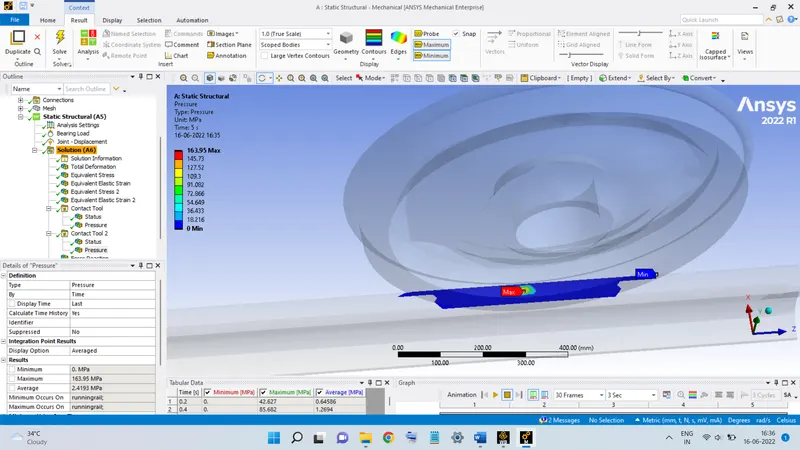
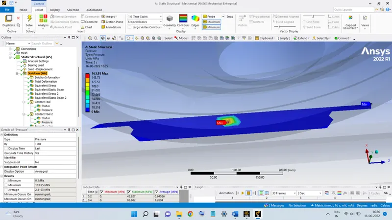
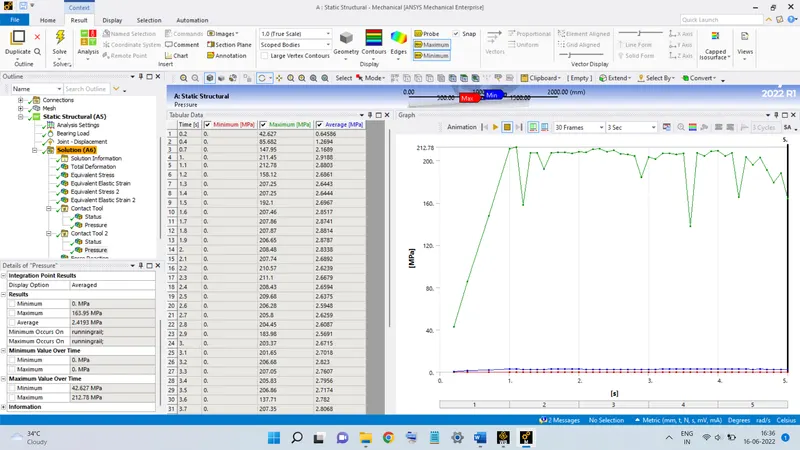
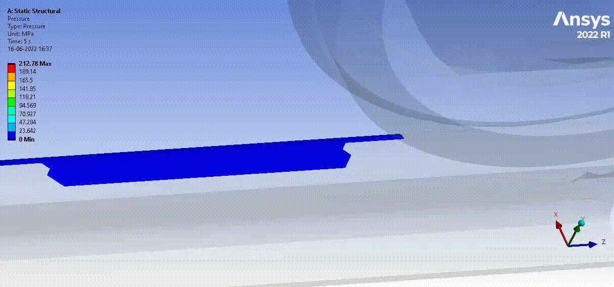
The pressure developed between the wheel and the track reaches a maximum value of 212.78 MPa.

Pressure between Wheel and Shaft:

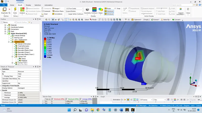
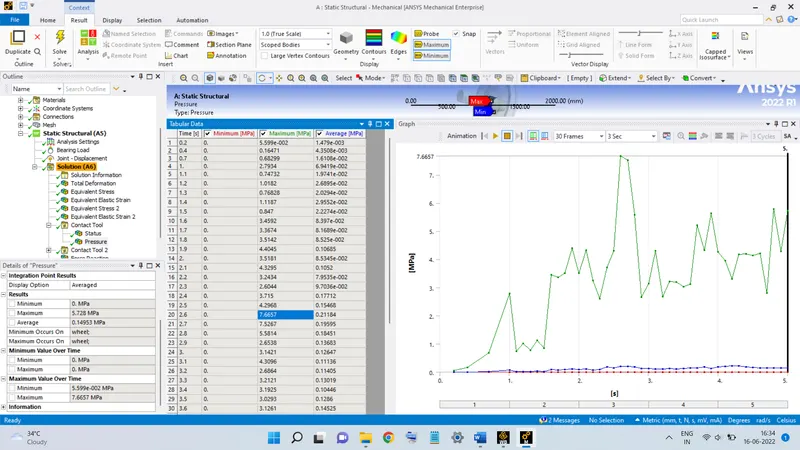
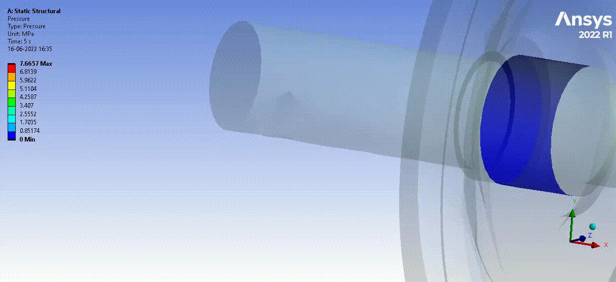
The maximum contact pressure between the shaft and the wheel is equal to 7.6657 MPa.

Life:

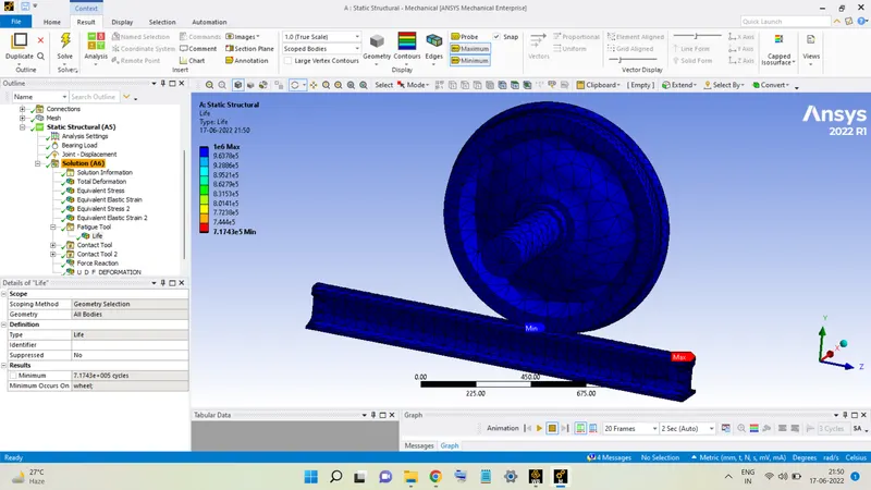
The minimum number of cycles without any failure for the given bearing load is equal to 7.1743 x 10⁵.

Reaction Force:

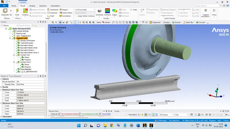
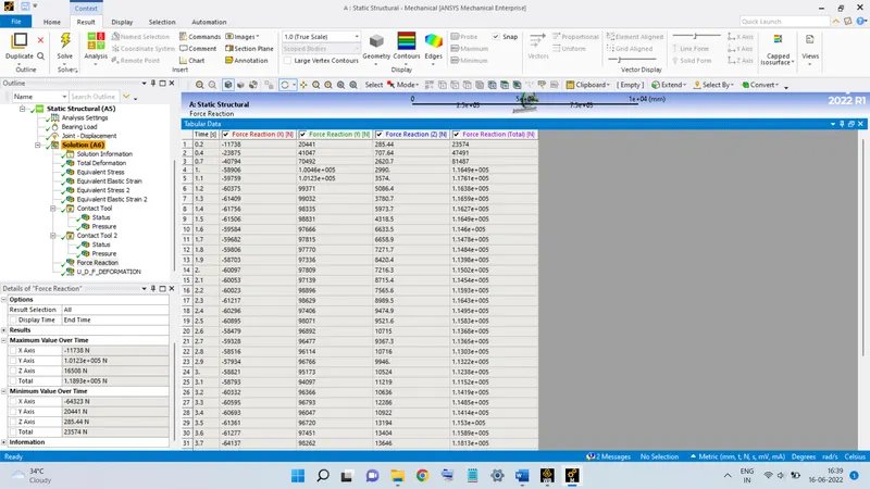
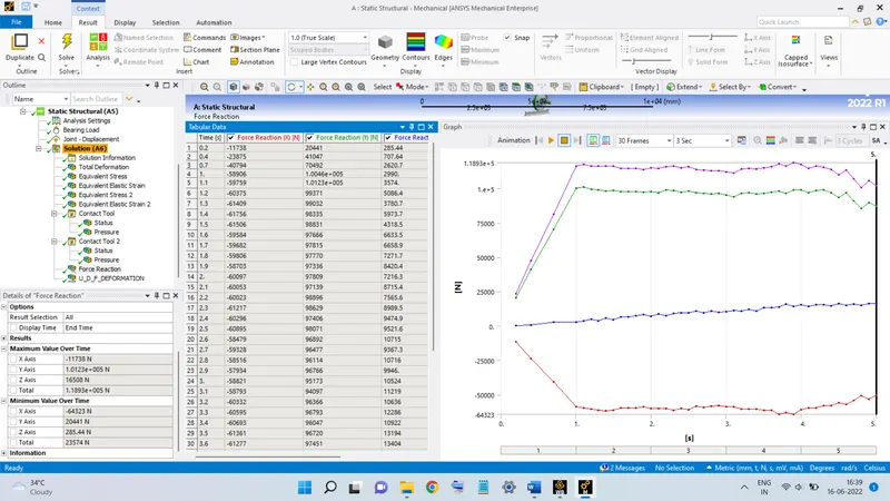
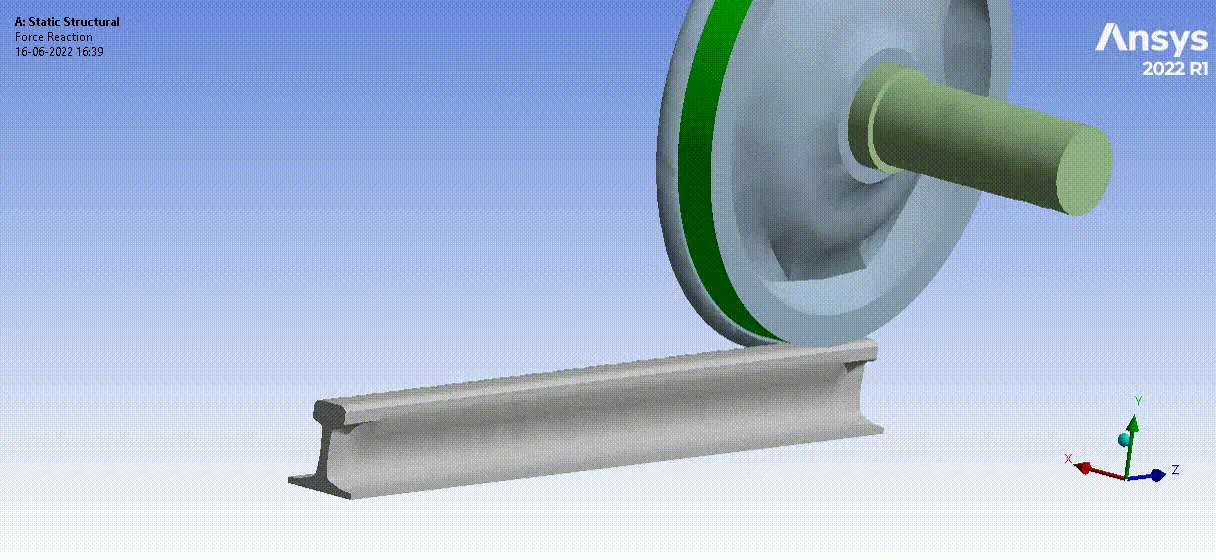
The reaction force value reaches a maximum value of 1.1893 x 10^5 N.

Total Deformation (User-Defined Result):

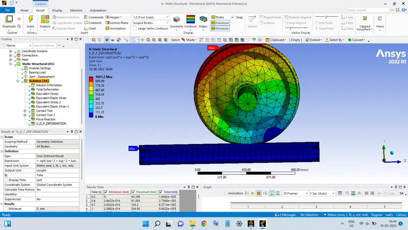
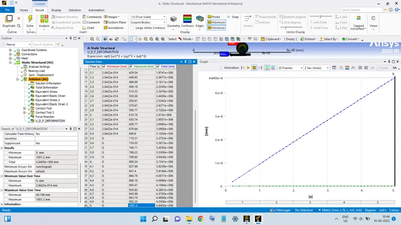
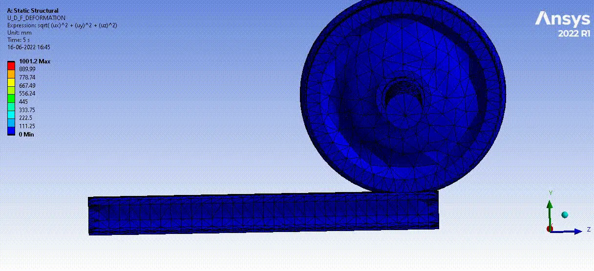
The above figures show the output results of the User-Defined Output (Total deformation). it is clear from the figures, that the output values of this quantity match with the Total Deformation output values.

CASE 1: Bearing Load of 500 kN

Equivalent Stress:

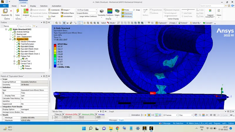
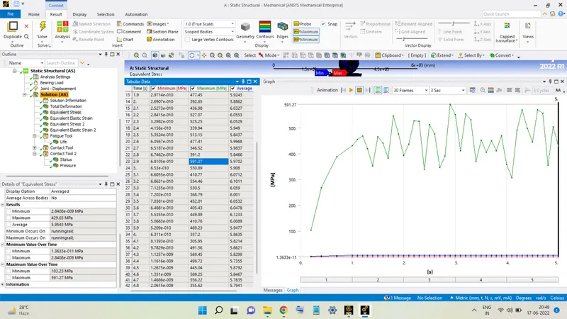
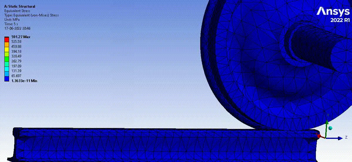
The maximum stress developed in the configuration is seen to be 591.27 MPa.

Equivalent Strain:

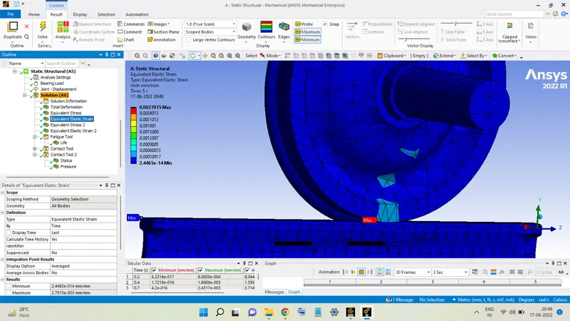
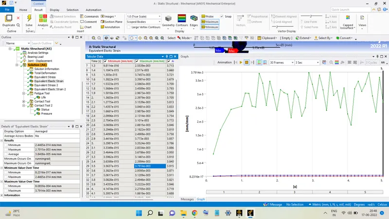
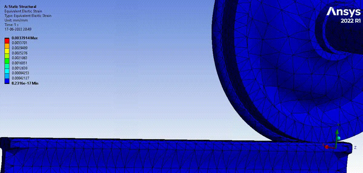
The maximum value of the strain is 3.7914 x 10^-3.

Stress in Wheel:

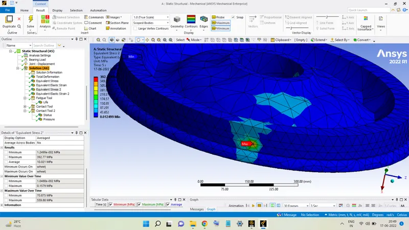
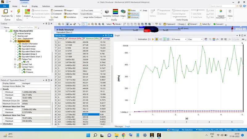
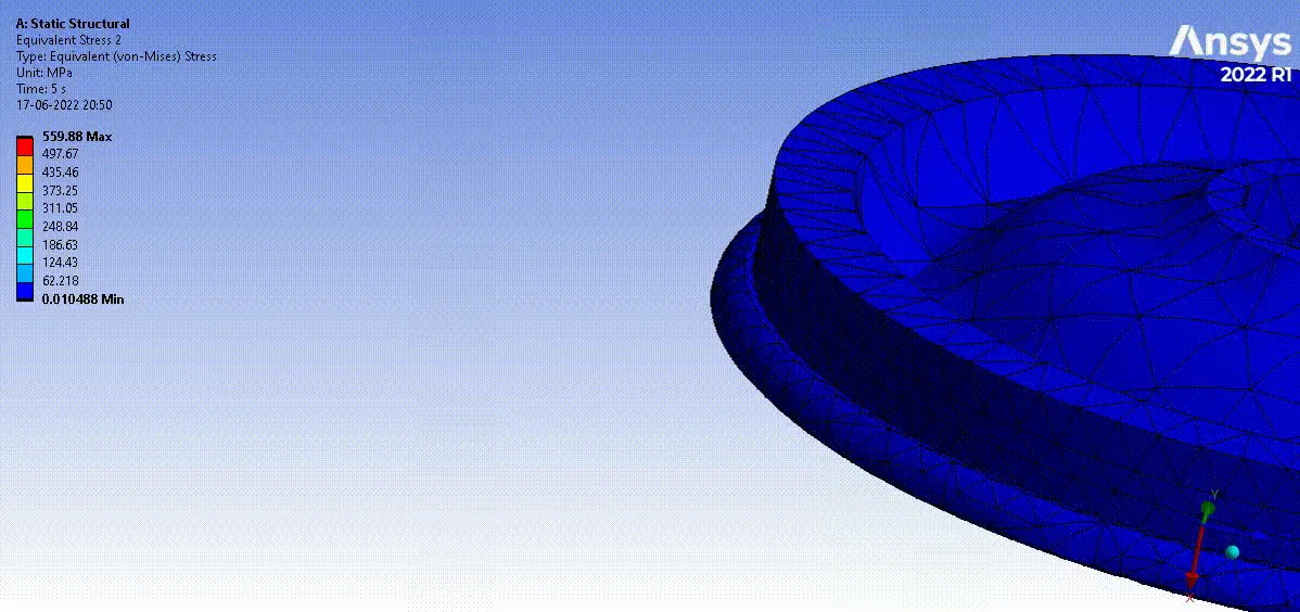
The maximum stress developed in the wheel alone is seen to be 559.88 MPa.

Strain in Wheel:

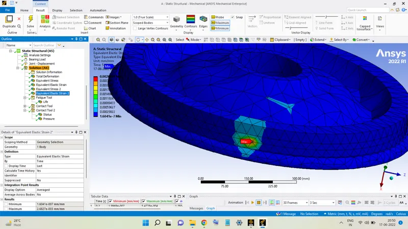
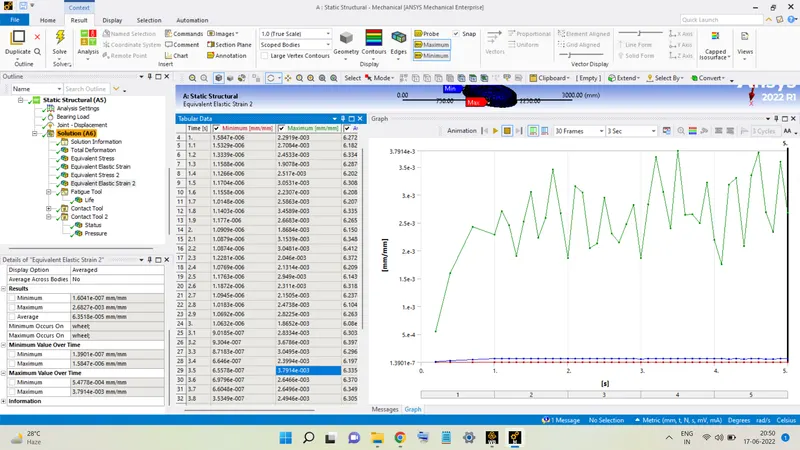
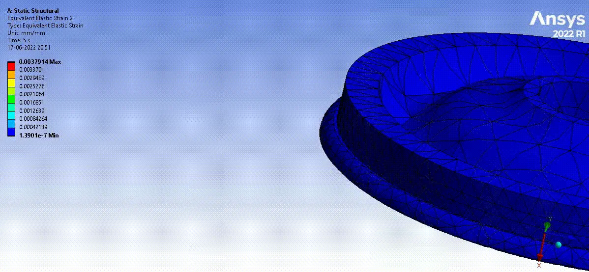
The maximum value of the strain in the wheel alone is 3.7914 x 10^-3.

Total Deformation:

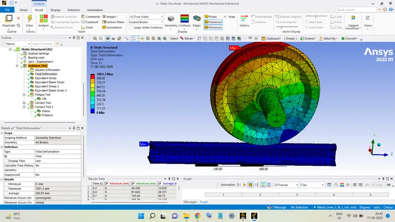
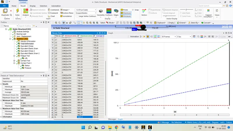
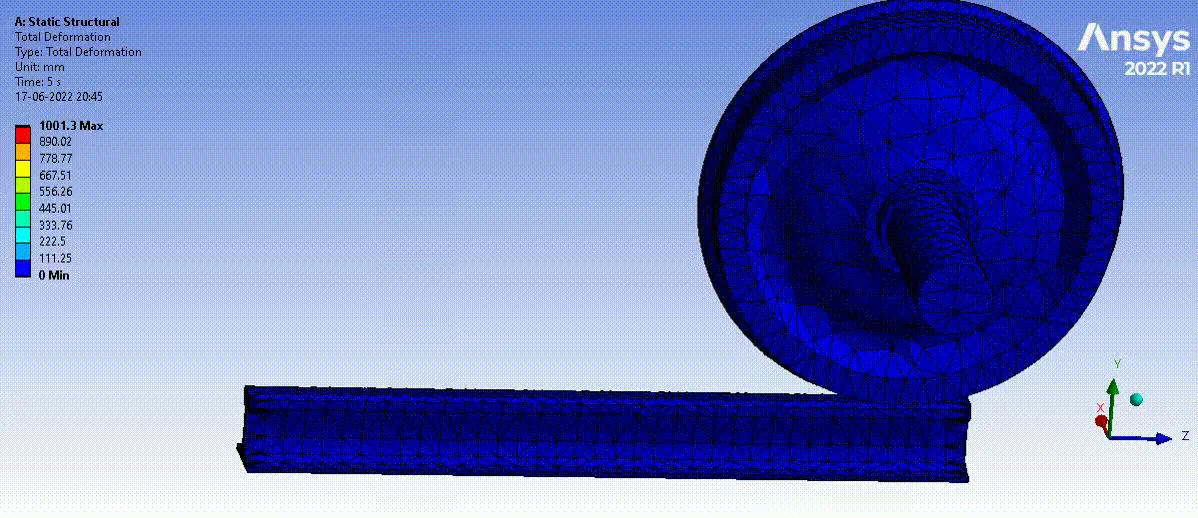
From the above figures, the maximum deformation is equal to 1001.3 mm.

Pressure between Wheel and Track:

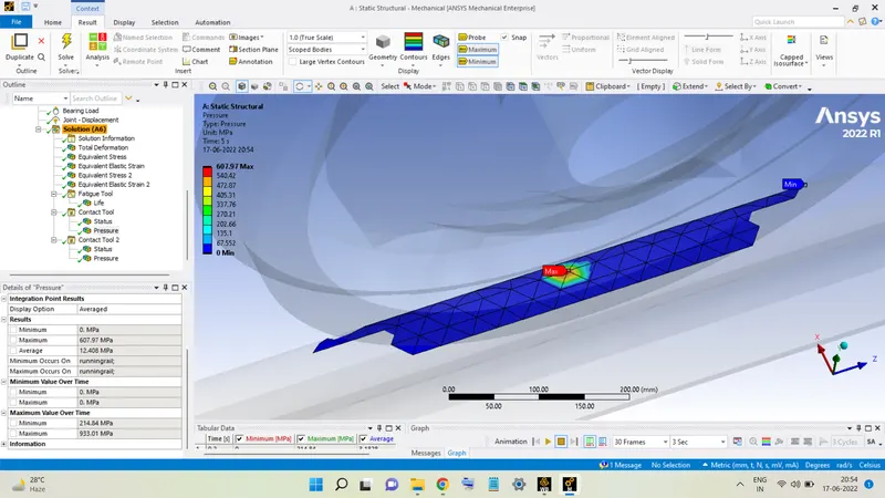
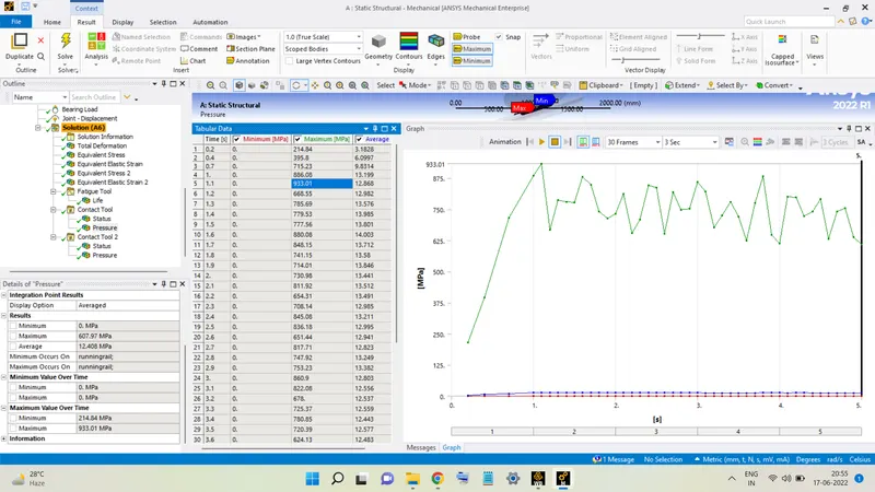
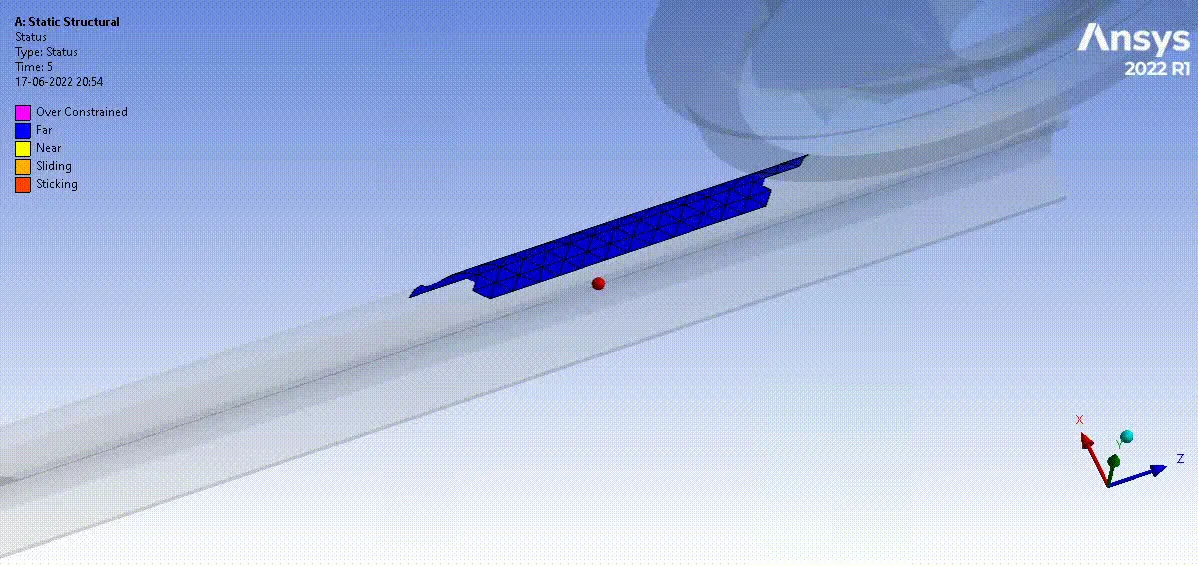
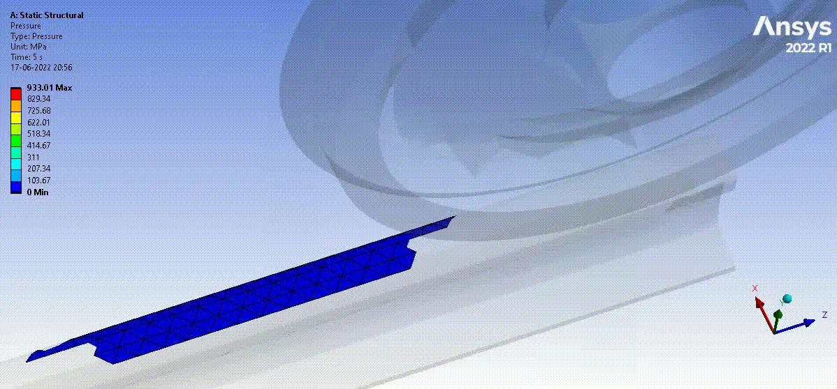
The pressure developed between the wheel and the track reaches a maximum value of 933.01 MPa.

Pressure between Wheel and Shaft:

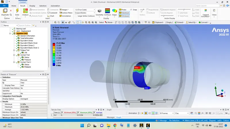
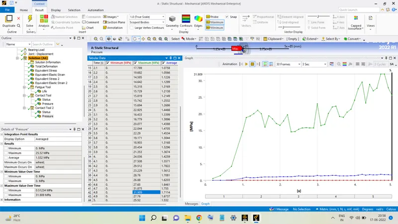
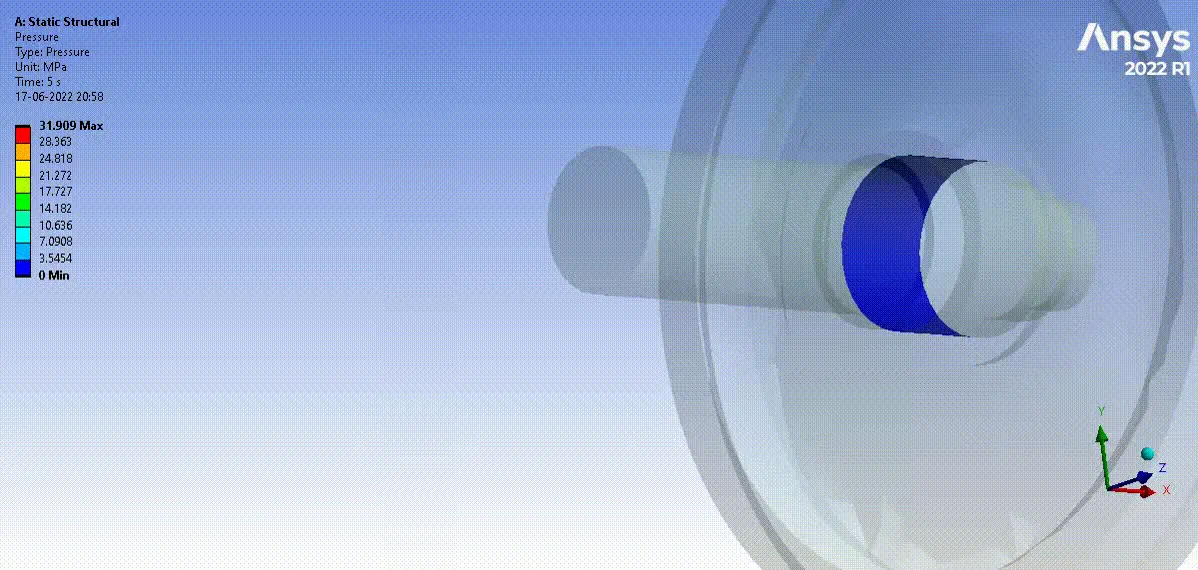
The maximum contact pressure between the shaft and the wheel is equal to 31.909 MPa.

Life:

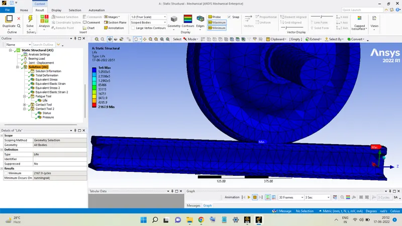
The minimum number of cycles without any failure for the given bearing load is equal to 2167.

Comparison:

	MAX. STRESS (MPa)	MAX. STRAIN	WHEEL STRESS (MPa)	WHEEL STRAIN	MINIMUM LIFE (NO. OF CYCLES)	DEFORMATION (mm)
CASE 1: Bearing Load = 100 kN	155.96	1.1925 x 10-3	152.71	1.1925 x 10-3	7.1743 x 105	1001.2
CASE 2: Bearing Load = 500 kN	591.27	3.7914 x 10-3	559.88	3.7914 x 10-3	2167	1001.3

From the above table, it can be said:

1. The stresses developed in the geometry are much higher for the second case.

2. Deformation in both cases is almost the same.

3. The minimum number of cycles reduces drastically in the second case.

4. Strain values are also higher in the second case.

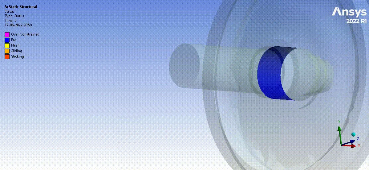
5. Also, the contact status results show sliding and sticking contact in some parts during the motion when subjected to the second case.

6. Thus, it can be said conclusively that the loading condition in CASE 2 is very severe and the wheel and track should not be put under such loading conditions.