Week 2 - Flow over a Cylinder.

AIM:

Simulate the flow over a cylinder and explain the phenomenon of Karman vortex street.

Questions :

PART-I

1. Simulate the flow with the steady and unsteady case and calculate the Strouhal Number for Re= 100.

PART-II

1. Calculate the coefficient of drag and lift over a cylinder by setting the Reynolds number to 10,100,1000,10000 & 100000. (Run with steady solver)
2. Discuss the effect of Reynolds number on the coefficient of drag. [ Results should be validated with any standard literature and error should be within 5 %]

Objectives :

1. In both approaches, show that the flow has converged. That is, what quantities or plots need to be looked at to determine that the flow has converged?
2. Plots of the coefficient of drag and lift.
3. Plots to show vortex shedding behind the cylinder.
4. Mention the referred material (Reference Paper or Fluid Mechanics Textbook) at the end of the challenge submission page.

Introduction :

When a fluid flows past a structure at a certain velocity, vortices known as Von Karman Vortex Street are created downstream of the body and detach periodically from either side of the body. Due to the alternating low pressure zone from either side of the structure, vibrations are induced in the structure. If the frequency of this vibration coincides with the natural frequency of the structure, it may lead to damage/failure of the structure. Vibrations induced due to vorticity occurs in many engineering structures such as bridges, transmission lines, offshore structures, thermos wells, engines, heat exchangers, marine cables, towed cables, etc. At very low Reynolds number, the streamlines of the resulting flow is perfectly symmetric. However as the Reynolds number is increased, the flow becomes asymmetric and leads to vortex shedding.

Karman vortex shedding :

Vortex shedding is a complex physical phenomenon in which a fluid such as air or water hits a bluff (as opposed to streamlined) body at certain velocities, vortices, known as Von Kármán vortex street, is created downstream of the body and detach periodically from either side of the body. The fluid flow over the object creates alternating low-pressure vortices on downstream side of the object. As the fluid flows to fill the low pressure zone, it produces a vibration at a specific frequency. If these vibration coincides with the natural frequency of the bluff body, it may lead to damage/fatigue failure of the body. The frequency of the vortices depends on the shape of the blunt body, and the velocity of the fluid flow or wind hitting this body.

Vortex shedding is a complex physical phenomenon in which a fluid such as air or water hits a bluff (as opposed to streamlined) body at certain velocities, vortices, known as Von Kármán vortex street, is created downstream of the body and detach periodically from either side of the body. The fluid flow over the object creates alternating low-pressure vortices on downstream side of the object. As the fluid flows to fill the low pressure zone, it produces a vibration at a specific frequency. If these vibration coincides with the natural frequency of the bluff body, it may lead to damage/fatigue failure of the body. The frequency of the vortices depends on the shape of the blunt body, and the velocity of the fluid flow or wind hitting this body.

Steps :

pre-processing steps 1-4

1. First of all we are going to start ansys work bench in which we going to start space claim in geometry section in which we have to create geometry of rectangular plate having cylinder wall at one point so first we create the circle in y plane taking the 0-axis at center point and diameter as 2m. before that we have to go In file > space claim option > units > and set lengths unit to meters after setting it to meter we then moves on to geometry again, now we select construction line and draw it 10*D from center of circle at left side which is our inlet point, and then taking another construction line 20*D from center of circle towards right side. Now we got our inlet points and outlet point so we now move to draw the rectangle plate so we taking the shortest side as 20*d and largest side we automatically get as 60m(from mid construction lines end we take 10*D up side and 10*D downside to get rectangle plate points).
2. Next we select the pull tool so we get the cylinder part cut from rectangle and then we delete those construction lines. Now as we end with our geometry part so we close the space claim.
3. Next we open mesh module in which first we defines boundaries like inlet, outlet, wall, and symmetry. Then we start to create mesh so first we right click on mesh and then click on mesh method and takes automatic method in which first we select body as our geometry in select geometry section , then in method we have to select triangular as we want triangular dominant mesh. Now as we want vortex shedding in model so we select maximum refinement for that we have to take minimum element size so we take 0.25m (before selecting this values we goes case by case and check the preferable mesh element size in which we first take 2m then, 1m, 0.5m and then finally we select 0.25m) next now we see there the circle edge is look alike 12 face polynomial hence we do the sizing of it for that we right click on mesh and select sizing then we select the edge of circle for geometry and click apply, and below that we select number of divisions as 36(simply because of 360 degree we assume that its good to go with 36 so that it can maintain specific 10 divisions gap, also good for engineering calculations)
4. Since the flow around the cylinder is important we want to take care of the region around the cylinder and for tis we use the tool named as inflation layer (inflation layer creates the body fitted mesh) for that we right click on mesh and select inflation layer then in geometry we select entire face and click apply, now next we defines the boundary condition by selecting the edge of circle, and we select first layer thickness in inflation option then going to number of layer we select 6 number of layer and first layer height to be 5e-3 , now clicking on generate mesh we gets the perfect body fitted mesh.
5. Next we close mesh module and start ansys fluent in which we first have to check our boundary conditions and then moving up we select laminar (as our Reynolds number is below or equal to 100) in viscous model, next we click on create material in which we go to fluent database and select air as our material and then copy it and name it as user material so we can make use of it in our model. But we changes the density here in this material as 1 and setting viscosity as 0.05 and as we have to simulate steady state for Reynolds number 100 so we put input velocity as 2.25m/s .
6. Now we have to create the monitor point so for that we goes to post processing going in create select the point clicking o that we give the mapping dimensions like our point is at 4*D at X-axis(8m) then we hit on ok.
7. Now next up we goes to residuals select the surface report > vertex average > selecting velocity as we want it for velocity > naming the residual “monitor point velocity” and same we creates lift and drag plots residuals.
8. Moving next we have to create the contours so we goes to result, then in plots and contour we click on contour then new > filling the data selecting the velocity > velocity magnitude select all the surfaces and then apply, same procedure for pressure contour too
9. Now next we create the animation file so we can see the vortex shed for that we goes to activities in solution and then hit on create solution animation and then select the velocity contour as we wants its animation and then goes to animation section and check the file created there
10. Now we initialize the solution and then run the calculation for 1000 iteration and we got the plots and results we see below

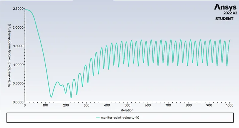
Fig 1. Steady state Monitor point velocity at RE=100

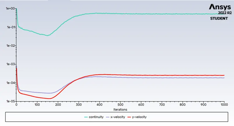
Fig2 : steady state scaled residuals for Re=100

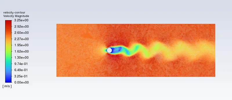
Fig 3: steady state vortex shedding for RE=100

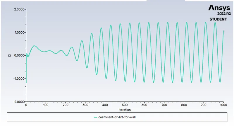
Fig 4: steady state lift coefficient for Re=100

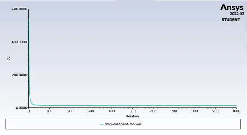
Fig 5: steady state drag coefficient for Re=100

in above plots we can see that in this steady state condition where Reynolds number is 100 the solution is looks converged at 450 iteration where we can see the moment is same no change in moment so we can say there the solution is get converged .

in this steady state case where the Reynold number varies the coefficient drag and coefficient lift also change as given in table below:

Reynolds number	Coefficient drag	Coefficient lift
10	0.339	8.606e-5
100	13.659	1.065
1000	758.30	359.89
10000	84618.819	44407.575
100000	8734202.3	5054963

Using this table we can clearly see that as the Reynolds number increase the drag is also going to increase,

now next we will try to change the Reynolds number and see how the residuals and all those plots perform.

Steady state case for Reynold number = 10

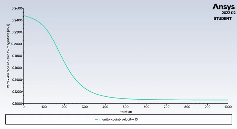
Fig 6. Monitor point velocity at re=10

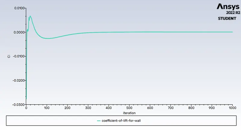
Fig 7: drag coefficient for re=10

Fig 8: coefficient lift for re=10

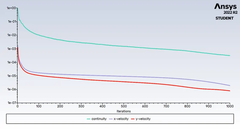
Fig 9: scaled residuals for re=10

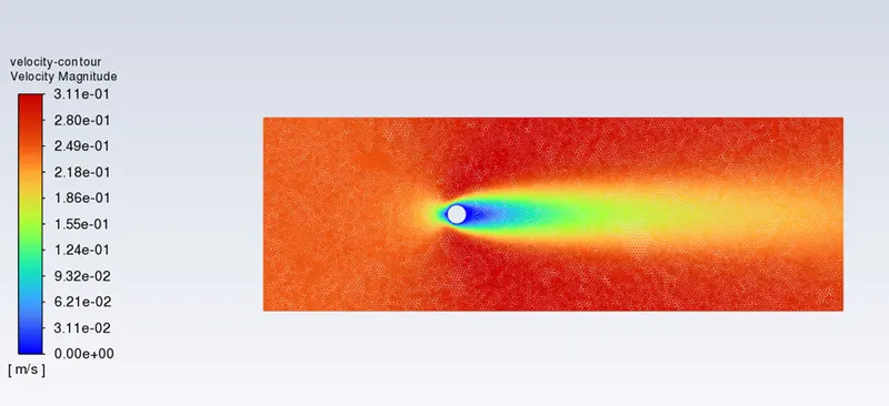
Fig 10: velocity contour for re=10

Steady state case for Reynold number = 1000

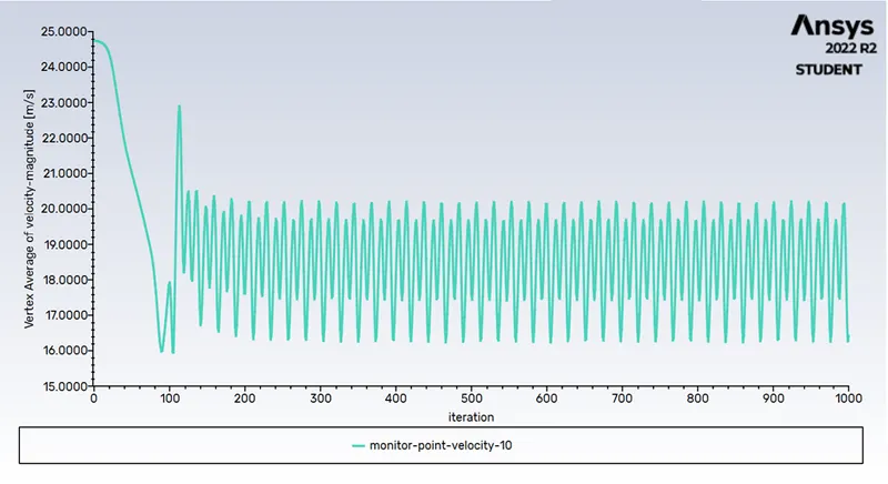
Fig 11: monitor point velocity re=1000

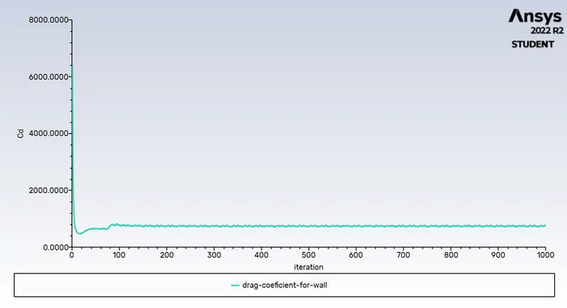
Fig 12: coefficient drag for re=1000

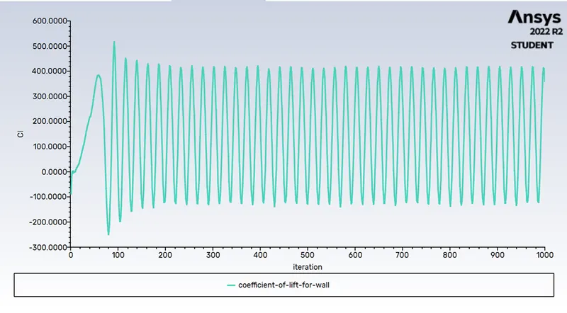
Fig 13: coefficient lift for re=1000

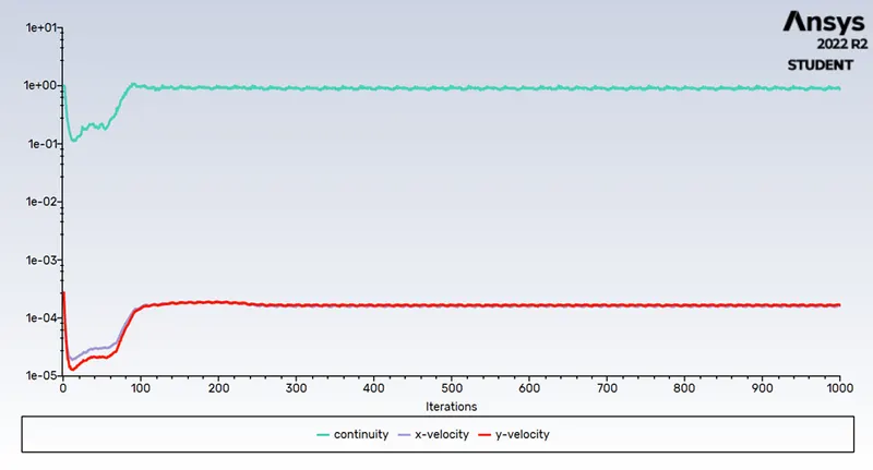
Fig 14: scaled residuals for re = 1000

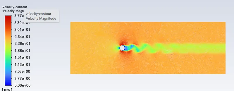
Fig 15: contour velocity for re=1000

Steady state case for Reynold number = 10000

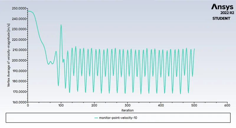
Fig 16: monitor point velocity at re=10000

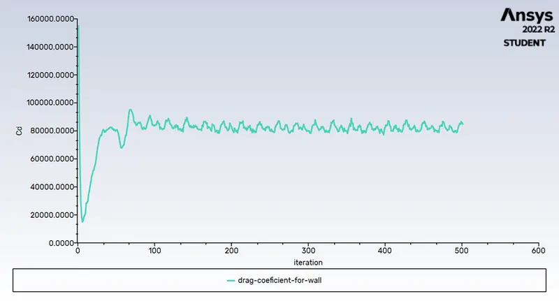
Fig 17: coefficient drag for re=10000

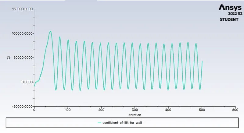
Fig 18: lift coefficient for re=10000

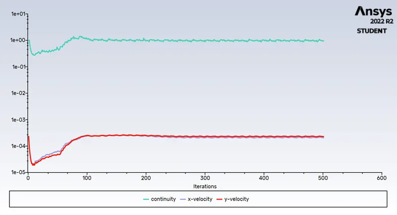
Fig 29: scaled residuals for re =10000

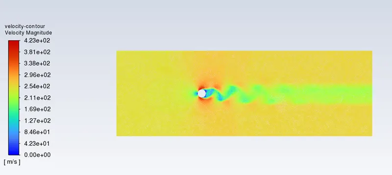
Fig 30: velocity contour for re=10000

Steady state case for Reynold number = 100000

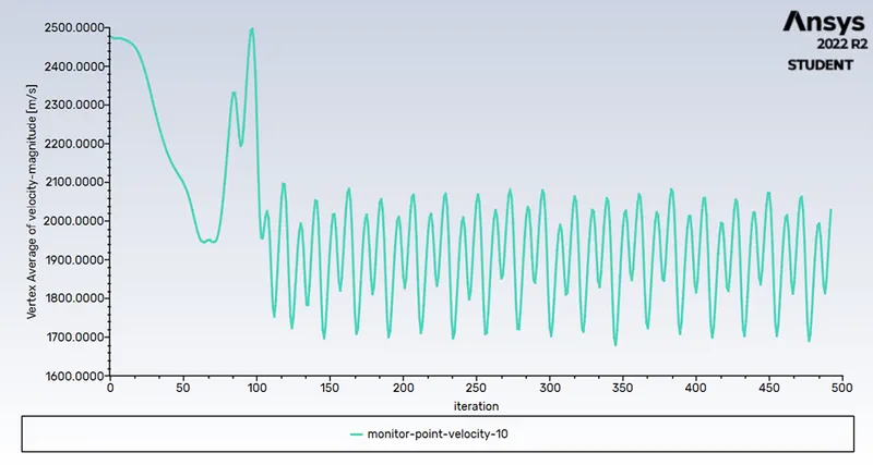
Fig 31: monitor point velocity for re=100000

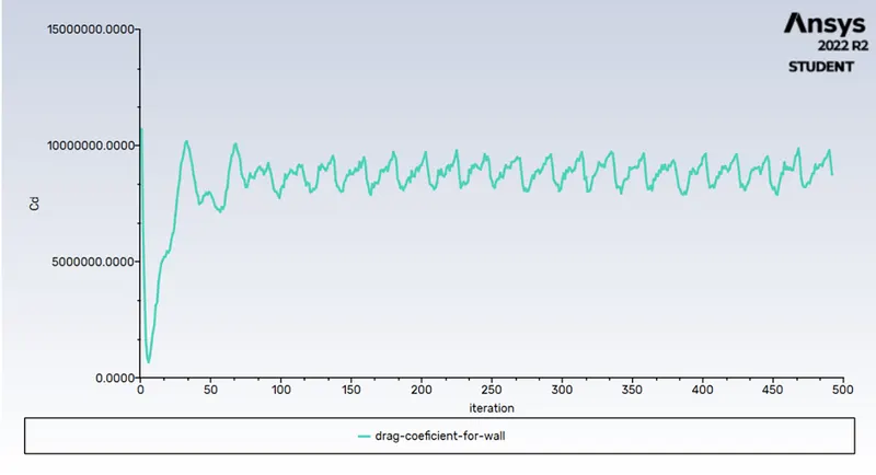
Fig 32: coefficient drag for re = 10000

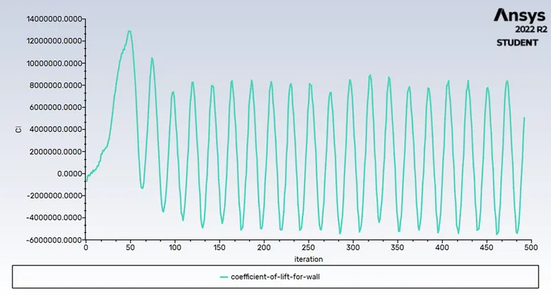
Fig 33: coefficient lift for re=100000

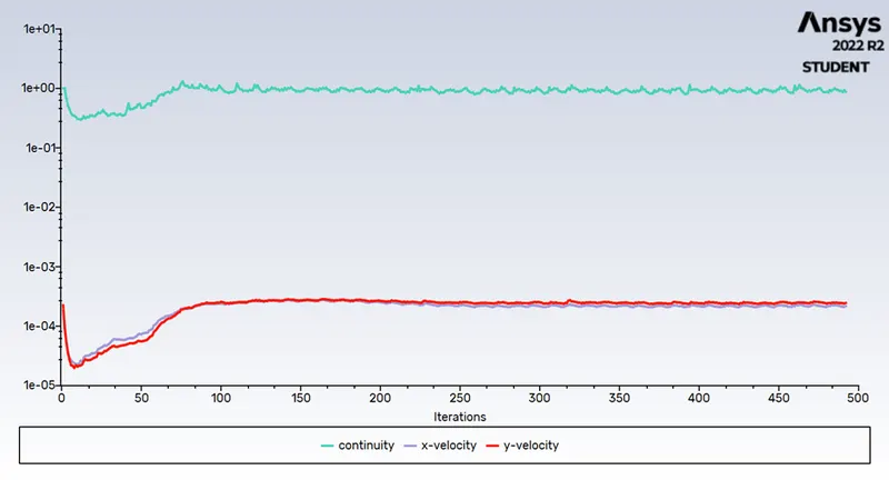
Fig 34: scaled residuals for re = 100000

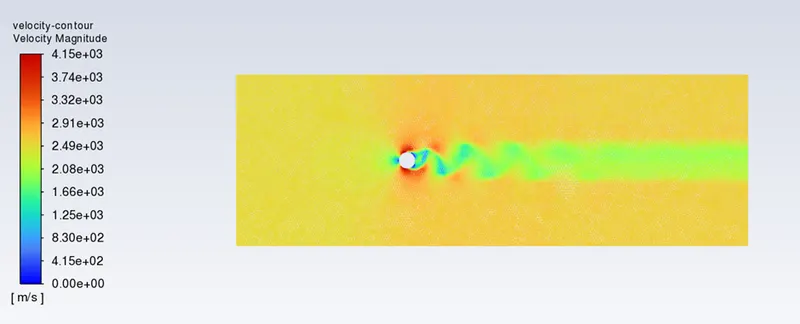
Fig 35: velocity contour

UNSTEADY STATE (transient)

Here pre-processing, plot and contour settings all are same as steady state or same as we done above we need just few changes in model to get unsteady state model here our velocity is for Reynolds number 100 liste of changes are below:

1. First of all we goes to physics tab and then there we select transient (between steady and transient) on basis of time step and flow time which we requires
2. Now same as above steady state here also we select the SIMPLE method as we have to deal with pressure and velocity
3. Now in steady state we need to type number of iterations but in transient as it is based on time here we requires to enter number of time steps and time step size for which we have one formula to select the time steps which we can see below using this we can calculate the time steps

Flow time = number of time steps * time step size

For example we have 150s flow time and we have to find time step size so we pick 2000 as number of time steps now after calculating 150/2000 we get 0.075 as size of time step

After runing calculation we get the data we want which is shown below :

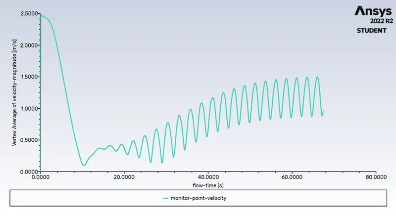
Fig 36. Monitor point velocity in unsteady state (re=100)

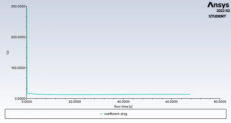
Fig 37. Coefficient drag for unsteady state (re=100)

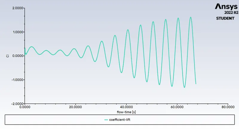
Fig 38.coefficient lift for unsteady state (re=100)

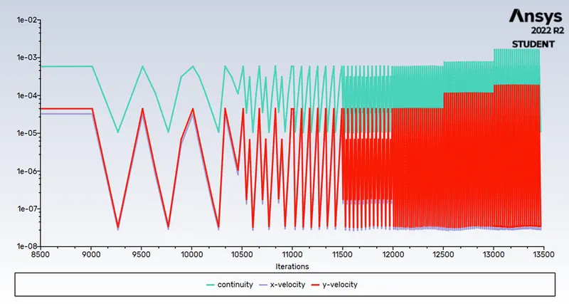
Fig 39. Scaled residuals for unsteady state (re=100)

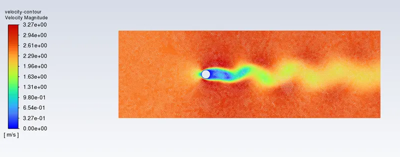
Fig 40. Velocity contour for unsteady state (re=100)

Calculate Strouhal number :

Strouhal number is dimensionless number describing oscillation flow mechanism

`st=(f*l)/v`

`st= (1.28 * 2)/2.25`

st= 1.024 for reynolds number 100 using above equation , where f is oscillation frequency , d is dameter or length to flow direction and v is flow velocity

Mention the referred material :

Referred material or fluid in our case is air but its viscosity and density changed we take density as 1 and viscosity as 0.05 kg/(m/s) at steady state with velocity according to Reynolds