Week 2 - Flow over a Cylinder.

STEADY VS UNSTEADY FLOW OVER A CYLINDER

AIM:

Simulate the flow over a cylinder and explain the phenomenon of Karman vortex street.

Simulate the flow with the steady and unsteady case and calculate the Strouhal Number for Re= 100.

Calculate the coefficient of drag and lift over a cylinder by setting the Reynolds number to 10,100,1000,10000 & 100000. (Run with a steady solver). Discuss the effect of the Reynolds number on the coefficient of drag. [ Results should be validated with any standard literature and error should be within 5 %]

INTRODUCTION:

One important class of fluid flow phenomena concerns the relative motion Between a fluid and the object submerged in it. The flow of air past a telephone wire or a bridge or the motion of an aircraft in a stationary atmosphere are some examples. The last flow situation is unaltered if the reference system with the aircraft is fixed so that it appears stationary with air blowing past with the same relative velocity. An idealized geometry of a long circular cylinder is considered for understanding such flow phenomena.

GOVERNING EQUATIONS AND THEORY:

Flow visualization is used to understand the flow past a long circular cylinder held with its axis normal to a steady stream. A direct experimental method involves the introduction of colored fluid at select points upstream of the cylinder and photographically records the motion of the particles.

As the flow velocity or the Reynolds number increases, changes are observed in the flow visualization mainly accounting for to drag vs velocity curve. At very low values of Reynolds Number (Re<<1), the lines indicating the paths of the fluid are shown in the figure below. The pattern is symmetrical. The velocity of fluid decreases as it approaches the body and becomes zero at contact with the cylinder. This point is called the STAGNATION POINT. The velocity increases from A to B and is maximum at B, and later decelerates to C (v=0), and accelerates further downstream.

accelerates further downstream.

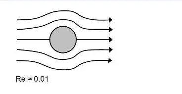
Fig. 1 Flow over a cylinder at low Re

As the flow velocity and Re increase, the development of fore-and-aft symmetry is observed. Two small regions are formed just behind the cylinder in which the fluid does not flow downstream as it does elsewhere, but whirls around in closed paths. These regions of recirculating flows are called ATTACHED EDDIES. One consequence of this phenomenon is that the flow no longer follows the contour of the body and is said to be SEPARATED. Another major effect that the increasing Re has on the flow picture is the modification of the region of disturbance to the flow stream. The distributed region upstream of the body and on its sides contract, while it elongates in the downstream direction. This region of disturbance downstream is termed WAKE.

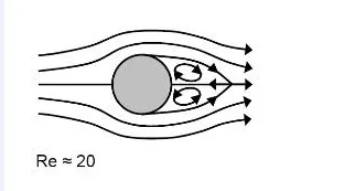
Fig. 2 Attached Eddies formation at Re=40

As Re is further increased the size of the two attached eddies increases. These eddies make the flow unstable, and consequently, when the Re exceeds a value (40) the eddies are shed from the surface and swept downstream. As the eddy is shed and swept away, new eddies are formed, shed, and swept downstream. The eddies on either side of the cylinder shed alternatively and create an unsteady, albeit periodic, wake flow. The wake of such a flow, with a series of staggered vortices, shed from either side of the cylinder and swept downstream by the flow is termed as KARMAN VORTEX STREET. It is noticed that for low values of Re, the velocity at a fixed point varies almost sinusoidally, but as Re increases the periodicity is lost.

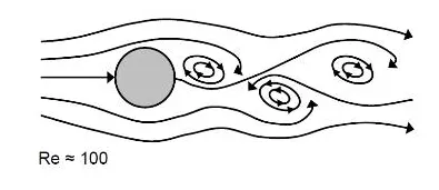
Fig. 3 Vortex Shedding at Re=100 and above

The lift coefficient is a dimensionless coefficient that relates the lift generated by a lifting body to the fluid density around the body, the fluid velocity, and an associated reference area. A lifting body is a foil or a complete foil-bearing body such as a fixed-wing aircraft. Cl is a function of the angle of the body to the flow, its Reynolds number, and its Mach number.

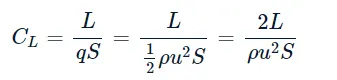
where L is the lift force, S is the relevant surface area and q is the fluid dynamic pressure, in turn, linked to the fluid density ρ, and to the flow speed u.

The drag coefficient is a dimensionless quantity that is used to quantify the drag or resistance of an object in a fluid environment, such as air or water. It is used in the drag equation in which a lower drag coefficient indicates the object will have less aerodynamic or hydrodynamic drag. The drag coefficient is always associated with a particular surface area.

Cd = 2*Fd/(ρ*(u^2)*A

where Fd is the drag force, which is by definition the force component in the direction of the flow velocity, ρ is the mass density of the fluid, u is the flow speed of the object relative to the fluid, A is the reference area.

In dimensional analysis, the Strouhal number is a dimensionless number describing oscillating flow mechanisms.

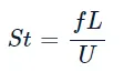
where f is the frequency of vortex shedding, L is the characteristic length and U is the flow velocity.

For large Strouhal numbers (order of 1), viscosity dominates fluid flow, resulting in a collective oscillating movement of the fluid "plug". For low Strouhal numbers (order of 10⁻⁴ and below), the high-speed, quasi-steady-state portion of the movement dominates the oscillation. Oscillation at intermediate Strouhal numbers is characterized by the buildup and rapidly subsequent shedding of vortices. It should be noted that the Strouhal number takes into consideration the frequency count

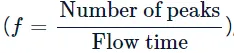, which is not applicable for a steady state simulation since no time physicality is considered in it. Strouhal number can be calculated only for transient solutions.

SOLVING AND MODELLING APPROACH:

For solving the problem statement, the following flow chart is followed:

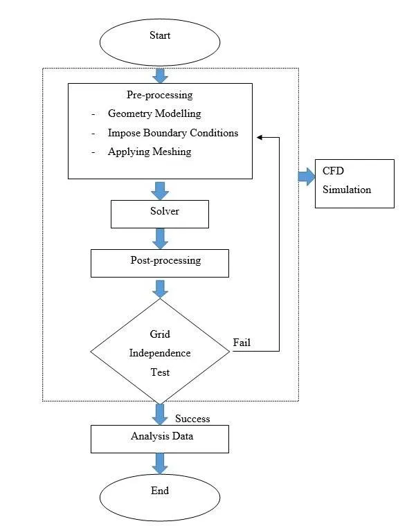
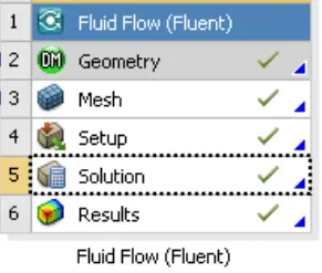
Fig. 4 ANSYS Solving Flow Chart

ANSYS involves the selection of a Fluent solver, input, and verification of Geometry, Meshing, Setup, Solutions, and Results. The Geometry is input in ANSYS Space Claim by drawing a 2D surface model of the required flow simulation. The mesh sizing and face naming are done while Meshing. The Setup section involves Mesh Checking, Turbulence Model selection, Solver type, velocity formulation and time (steady or transient state), Output report files, Material selection, and Initial and Boundary conditions. The Results section is used for the visualization of the output in a GUI.

The modeling approach as stated in the problem statement includes both STEADY and TRANSIENT STATE simulation to observe the Strouhal Number. The solution is originally a transient state simulation output, but the desired vortex shedding can be observed in a steady state solution at higher Re values. The k-ε model is used to run the transient state simulation.

PRE-PROCESSOR AND SOLVER SETTINGS:

GEOMETRY:

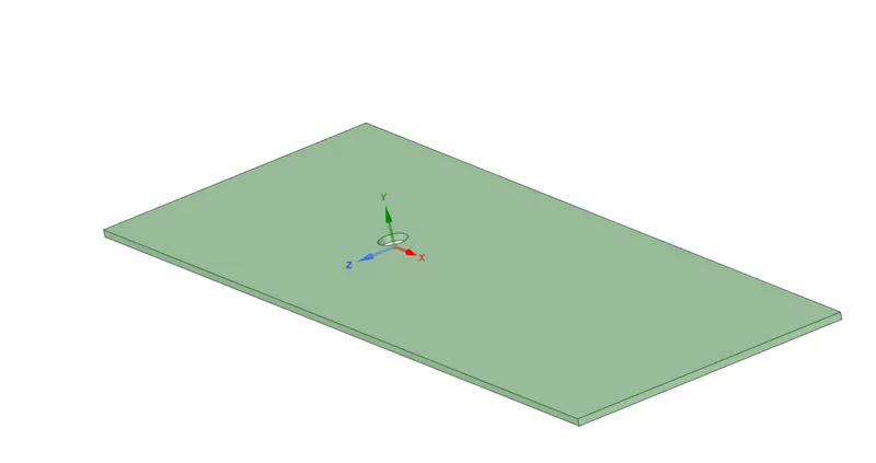
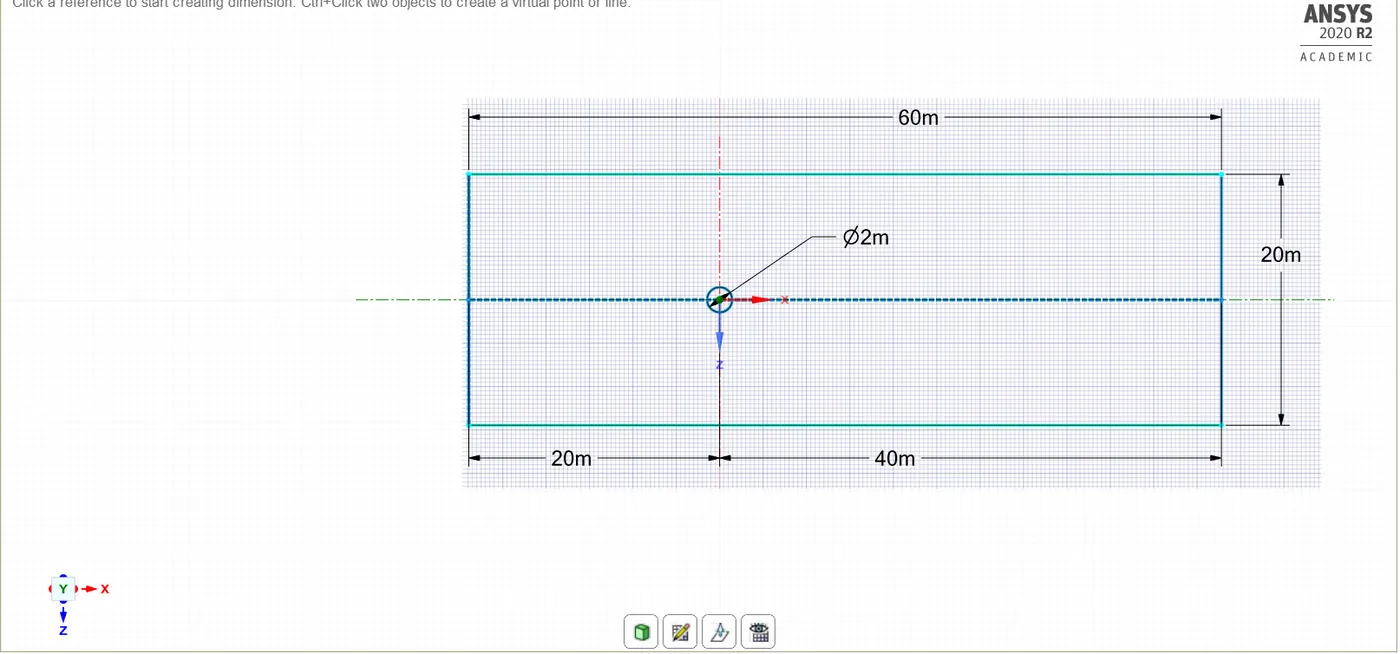
The geometry is sketched in SpaceClaim. On the XZ plane, a D=2m diameter circle is drawn and enclosed with an inlet side at 10D upstream and an outlet side at 20D downstream. The symmetry condition was used on the other two boundaries at 5D from the center of the circle. After the geometry is drawn the circle part is deleted and the geometry is extruded outside to create a body. This is done because, now all the fluid flow is being visualized in the body left, and that is what is required for the simulation.

MESH:

The Meshing tab is opened, and when Generate Mesh is used, a mixture of quadrilaterals and triangles is input into the mesh domain. The Element size of the Mesh is set to 0.3m. To create a uniform mesh, a New Method is inserted into the mesh, and the Triangles method is selected. To improve the sizing on the edge of the circle, the Sizing option is inserted in the Mesh and the Number of Divisions is increased to 36

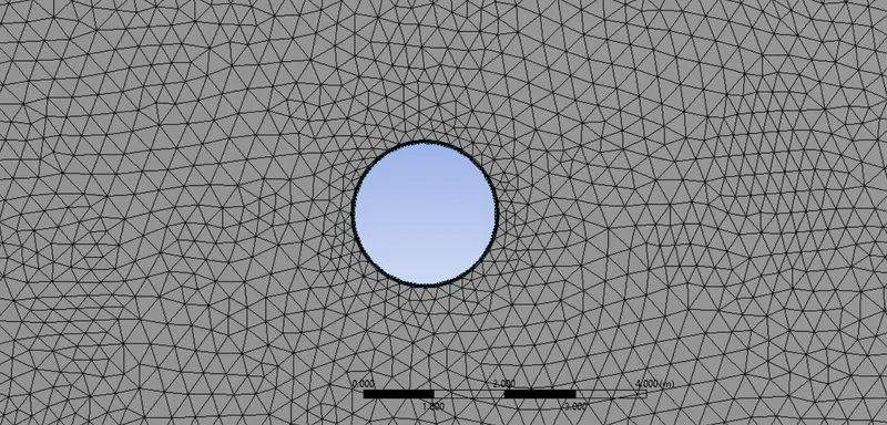
An Inflation Layer is added to the mesh to better visualize the flow at the surface of the circle. The First Layer thickness is set to 5mm, the number of layers to 5, and the successive percentage increase in thickness to 20%.

Later the respective sides are selected and named Inlet (upstream-left), Outlet (downstream-right), Wall (Circle circumference), and Symmetry Boundary (Above and below the circle) accordingly.

SETUP:

The simulation is run and compared for both steady and unsteady states. The Re is set to 10,60,100,1000, and 10000 for steady-state comparison, and the Strouhal number is computed for the transient state simulation (Re=100). Therefore for the respective case, the solver is set to Pressure Based Type, Absolute Velocity Formulation, and the Time State (Steady/Unsteady). The viscous model for both cases is set to Laminar. A new user material is defined with μ=0.02Pa.s">μ=0.05 Pa.s(case specific) and Density of 1 kg/m^3. A No-Slip boundary condition is employed on the cylinder wall and a Symmetry condition is set for the edges above and below the cylinder.

To observe the velocity variation a Vertex Average is plotted to a monitor point 8m (4xDiameter) downstream from the center of the cylinder. To observe the velocity development in the whole domain, a velocity contour plot is observed for each case.

Comparison:

Case 1:

Steady state at Re = 10, viscosity of 0.05 Pa s, Density 1 kg/m^3, and inlet velocity at 0.25 m/s.

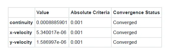
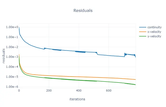
It can be seen from the figure given that after running the solver for about 700 iterations the solution was converged

Residual while converging the solution:

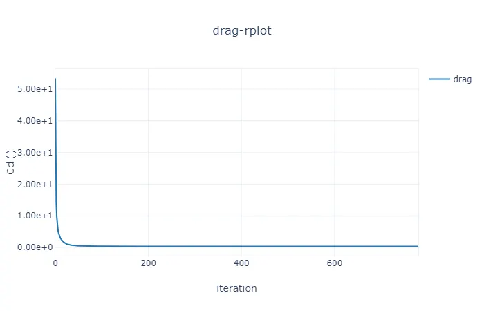
Drag coefficient:

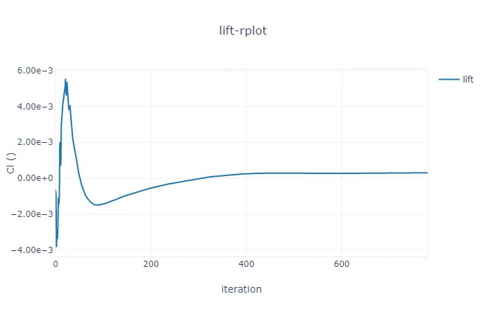
Lift coefficient:

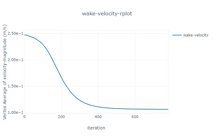
Velocity at the monitor point:

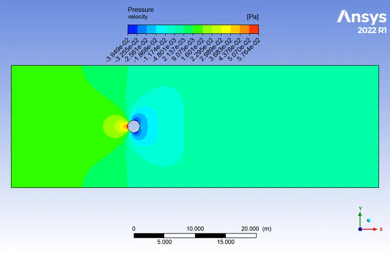
Pressure contour:

Velocity contour and vector:

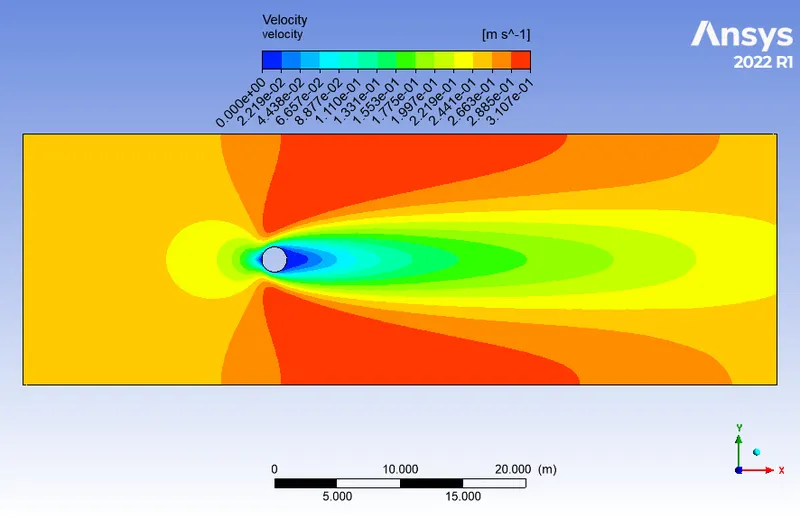
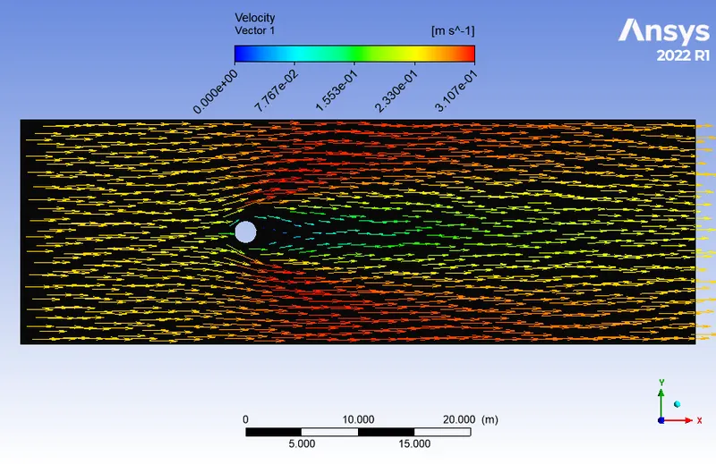
It can be seen from the pressure and velocity contour that no vortices are formed at Re 10 and the flow of the air is laminar in nature.

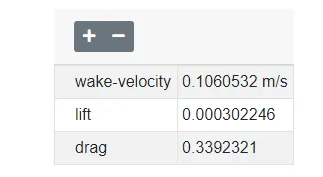
Results:

Case 2:

Steady state at Re = 60, viscosity of 0.05 Pa s, Density 1 kg/m^3, and inlet velocity at 1.5 m/s.

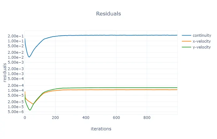
As at Re = 60 which is more than Re = 47, the vortices initiate to form and so the continuity equation does not converge due to fluctuation in the velocity.

Residual while converging the solution:

Drag coefficient:

Lift coefficient:

Velocity at monitor point:

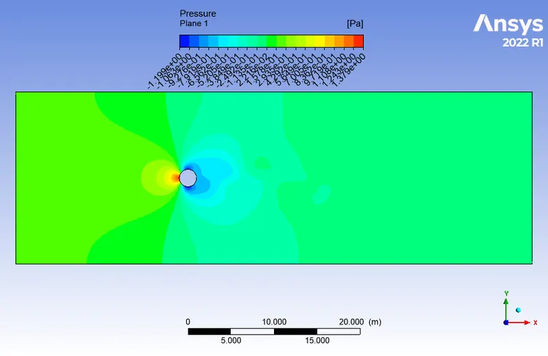
Pressure contour:

Velocity contour and vector:

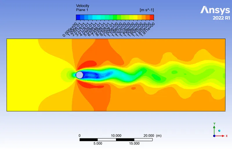
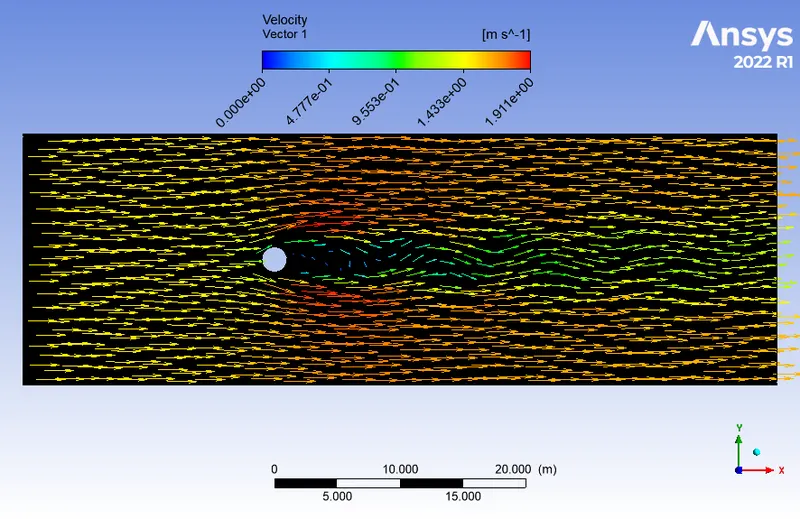
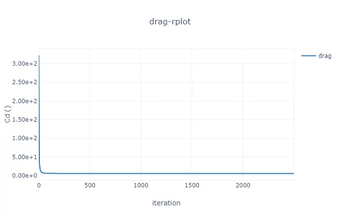
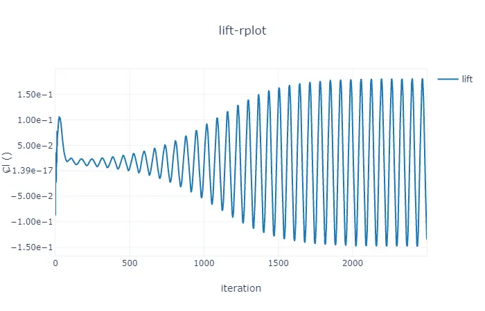
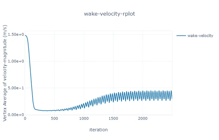
Here from the velocity contour, vector and plot it can be observed that small vortices are formed and a wakefield after the pipe can be observed downstream of the flow. And the vortex Karman street width widest at lower Re values.

Results:

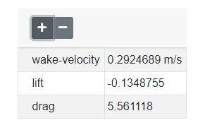
The definitions results provided in the figure above are incorrect as the lift coefficient and velocity in the wakefield keep on fluctuating as the vortices are sheded but the drag coefficient remains constant the value of the drag coefficient is accurate.

Case 3:

Steady state at Re = 100, viscosity of 0.05 Pa s, Density 1 kg/m^3, and inlet velocity at 2.5 m/s.

As at Re = 100 which is more than Re = 47, the vortices initiate to form and so the continuity equation does not converge due to fluctuation in the velocity.

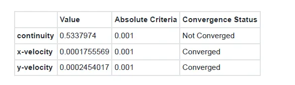
Residual while converging the solution:

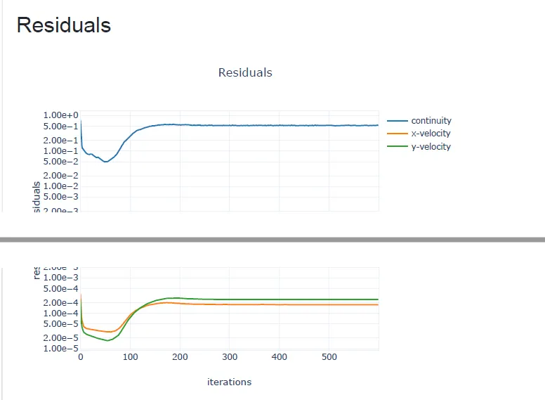
Drag coefficient:

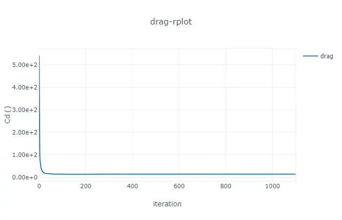
Lift Coefficient:

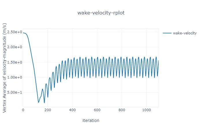
Velocity at the monitor point:

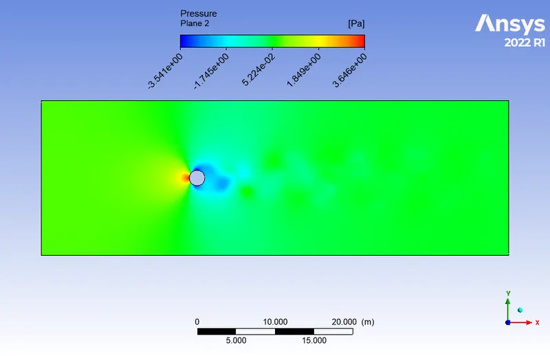
Pressure contour:

Velocity contour, vector and animation:

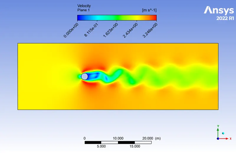
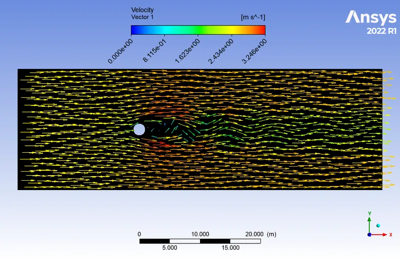
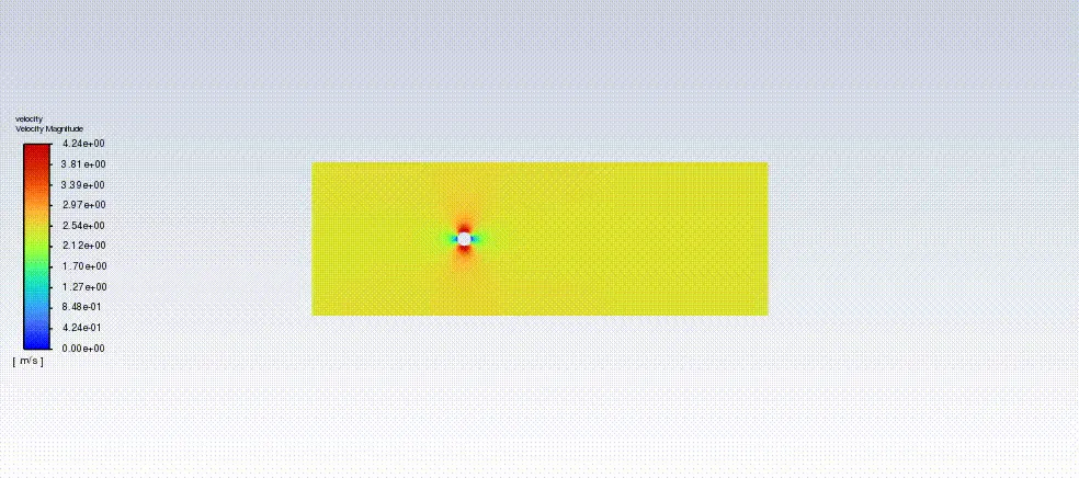
From the contours, vector diagram and plot provided above it can be seen that the wake region formed at a higher velocity is shorter and more vortices are formed with a greater magnitude of vacuum in the wake region. And since the velocity is increased the vortex Karman street got narrower.

Results:

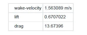
The definitions results provided in the figure above are incorrect as the lift coefficient and velocity in the wakefield keep on fluctuating as the vortices are sheded but the drag coefficient remains constant the value of the drag coefficient is accurate.

Case 4:

Transient state at Re = 100, viscosity of 0.05 Pa s, Density 1 kg/m^3, and inlet velocity at 2.5 m/s.

Time stamp = 0.1sec per iteration

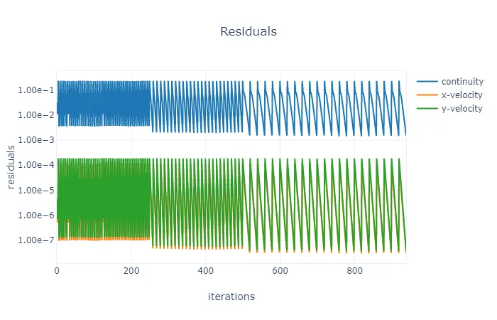
As at Re = 100 which is more than Re = 47, the vortices initiate to form and so the continuity equation does not converge due to fluctuation in the velocity.

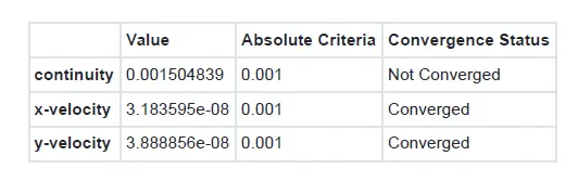
Residual while converging the solution:

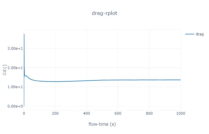
Drag Coefficient:

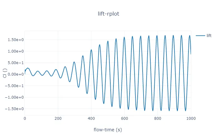
Lift Coeffcient:

Strouhal number calculation:

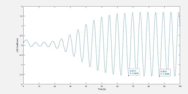
as Strouhal number = (frequency*Characterstic length)/Flow velocity

here from the plot of lift coefficient, it can be seen that 4 cycles are repeated between time 67.2 sec and 86.9sec so frequency = 4/(86.9-67.2) = 0.20304 Hz

and as the diameter of the pipe is 2m so characteristic length is 2

and inlet flow velocity for this case is 2.5m/s

so Strouhal number = (0.20304*2)/2.5 = 0.16243

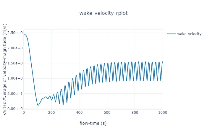
Velocity at the monitor point:

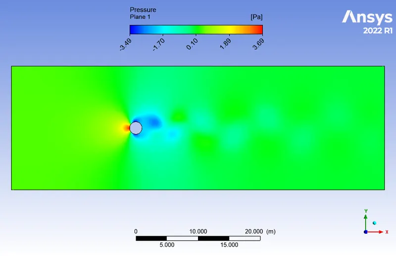
Pressure contour:

Velocity contour and vector:

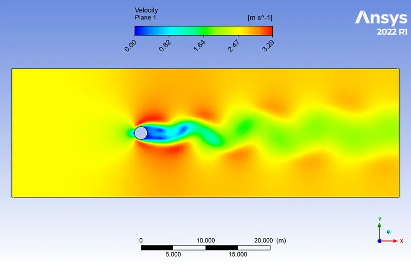
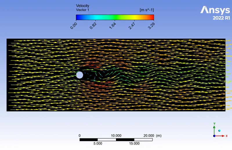
From the contours, vector diagram and plot provided above it can be seen that the wake region formed at a higher velocity is shorter and more vortices are formed with a greater magnitude of vacuum in the wake region. Here the contour and vector are almost similar to the steady state contour at Re = 100.

Results:

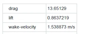
The definitions results provided in the figure above are incorrect as the lift coefficient and velocity in the wakefield keep on fluctuating as the vortices are sheded but the drag coefficient remains constant the value of the drag coefficient is accurate.

Case 5:

Steady state at Re = 1000, viscosity of 0.05 Pa s, Density 1 kg/m^3, and inlet velocity at 25 m/s.

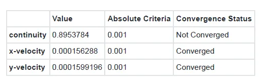
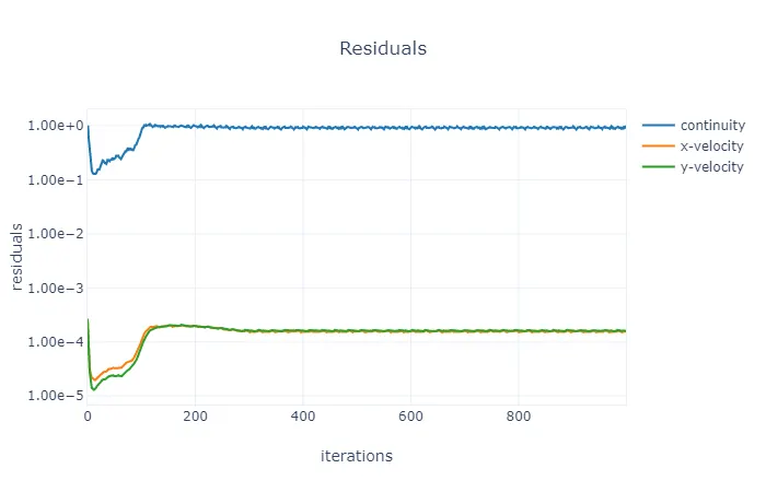
As at Re = 1000 which is more than Re = 47, the vortices initiate to form and so the continuity equation does not converge due to fluctuation in the velocity.

Residual while converging the equation:

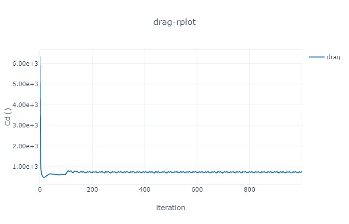
Drag coefficient:

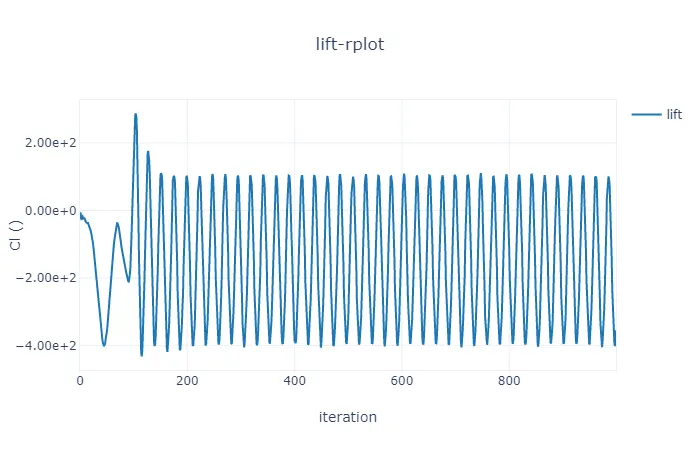
Lift Coeffcient:

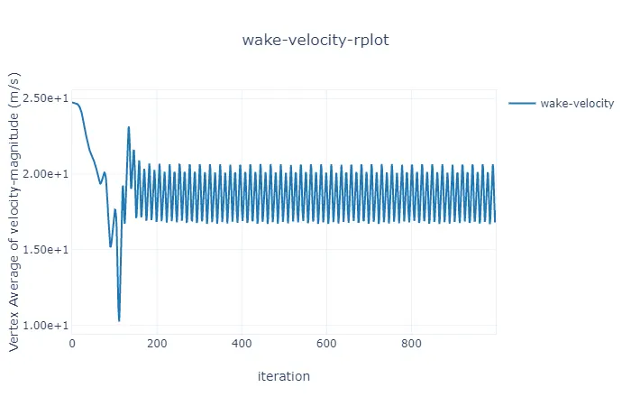
Velocity at the monitor point:

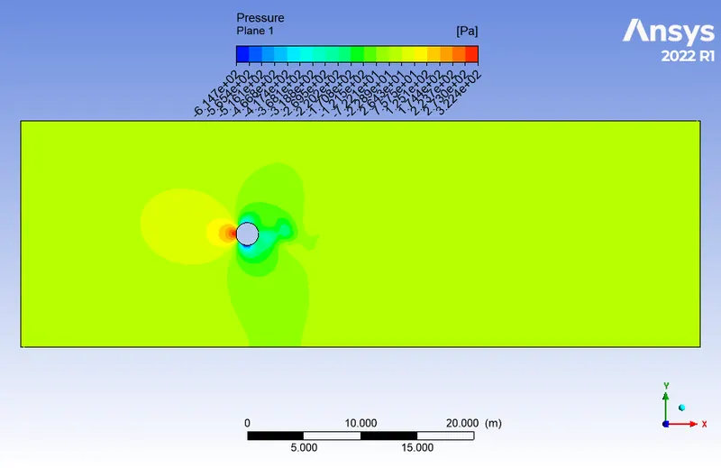
Pressure contour:

Velocity contour and vector:

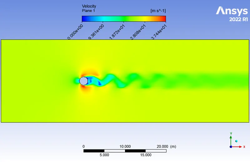
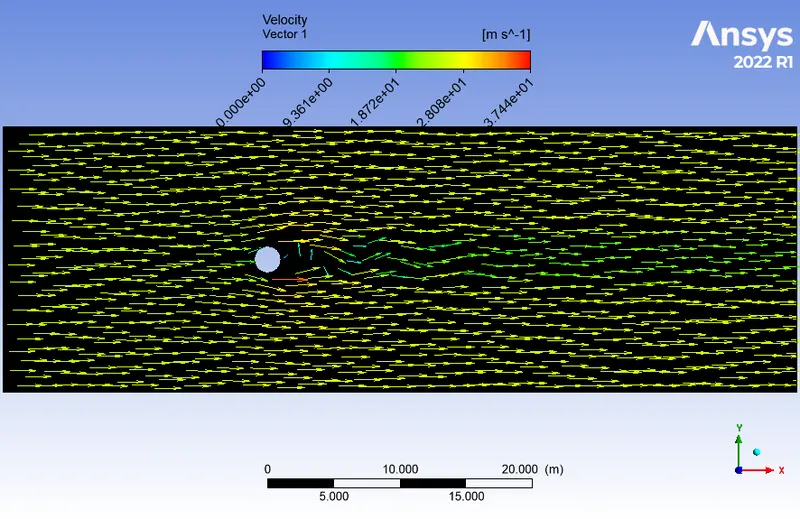
From the contours, it can be observed that as the velocity of the inlet fluid increases the wake region is reduced and the flow becomes more streamlined avoiding the obstruction of the pipe and the vortex Karman street width being narrowed down.

Results:

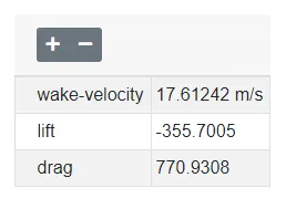
The definitions results provided in the figure above are incorrect as the lift coefficient, velocity, and drag coefficient are inaccurate as it can be seen from their respective plots that their values keep on fluctuating and so the latest value at the time when the iterations terminated are being displayed but since at the higher velocity the change in the drag coefficient is not significant it can be approximated from the obtained results.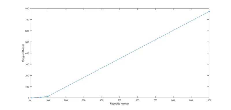

Case 6:

Steady state at Re = 10000, viscosity of 0.05 Pa s, Density 1 kg/m^3, and inlet velocity at 250 m/s.

As at Re = 10000 which is more than Re = 47, the vortices initiate to form and so the continuity equation does not converge due to fluctuation in the velocity.

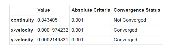
Residual while converging the equation:

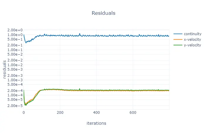
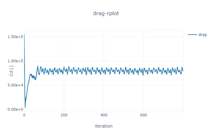
Drag Coefficient:

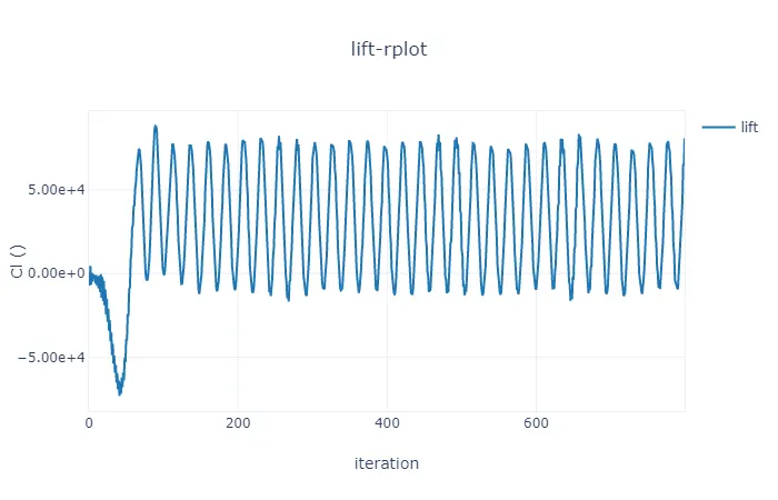
Lift coefficient:

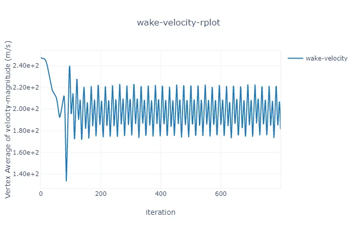
Velocity at the monitor point:

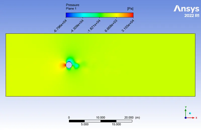
Pressure contour:

Velocity contour and vector:

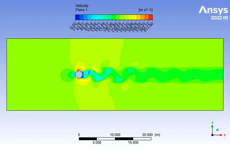
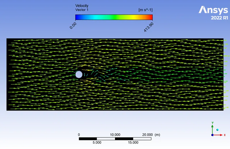
From the contours, it can be observed that as the velocity of the inlet fluid increases the wake region is reduced and the flow becomes more streamlined avoiding the obstruction of the pipe and the vortex Karman street width being narrowed down.

Results:

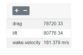
The definitions results provided in the figure above are incorrect as the lift coefficient, velocity, and drag coefficient are inaccurate as it can be seen from their respective plots that their values keep on fluctuating and so the latest value at the time when the iterations terminated are being displayed but since at the higher velocity the change in the drag coefficient is not significant it can be approximated from the obtained results.

Comparison of the drag force at various Reynolds number in the steady state condition:

Preferred material for instability:

In order to prevent the unwanted vibration of cylindrical bodies, a longitudinal fin can be fitted on the downstream side, which, provided it is longer than the diameter of the cylinder, will prevent the eddies from interacting, and consequently they remain attached. Obviously, for a tall building , the relative wind could come from any direction. For this reason, helical projections resembling large screw threads are sometimes placed at the top, thereby discouraging the alternate shedding of vortices. Another countermeasure with tall buildings is using variation in the diameter with height, such as tapering - that prevents the entire building being driven at the same frequency. For example, spiral added to the chimney to avoid vortex shredding

References:

https://web.calpoly.edu/~kshollen/ME554/Labs/validation_example.pdf