Week 2 - Flow over a Cylinder.
Steady Vs Unsteady flow over a cylinder
Objective:
Part I:
- Simulate the flow over a cylinder and explain the phenomenon of Karman vortex street.
- Simulate the flow with the steady and unsteady case and calculate the Strouhal Number for Re= 100.
Part II:
- Calculate the coefficient of drag and lift over a cylinder by setting the Reynolds number to 10,100,1000,10000 & 100000. (Run with steady solver)
- Explore the effect of Reynolds number on the coefficient of drag. [ Results should be validated with any standard literature and error should be within 5 %]
Solution:
PART I
Von Karman Vortex Street:
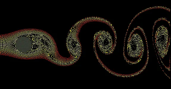
Von Karman vortex street is a repeating pattern of swirling vortices, caused by a process known as vortex shedding, which is responsible for the unsteady separation of flow of a fluid around blunt bodies.
Vortex shedding is a phenomenon, when the wind blows across a structural member, vortices are shed alternately from one side to the other, and where alternating low-pressure zones are generated on the downwind side of the structure giving rise to a fluctuating force acting at right angles to the wind direction. This is clearly visible in the below fig.
Geometry:
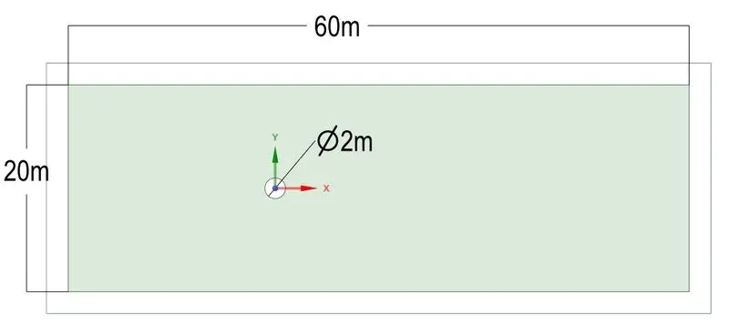
Geometry is created using Spaceclaim with the dimensions as shown in the image.
Meshing:
Meshing is done in several steps.
1. A triangular mesh is created using Methods option.
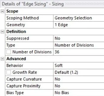
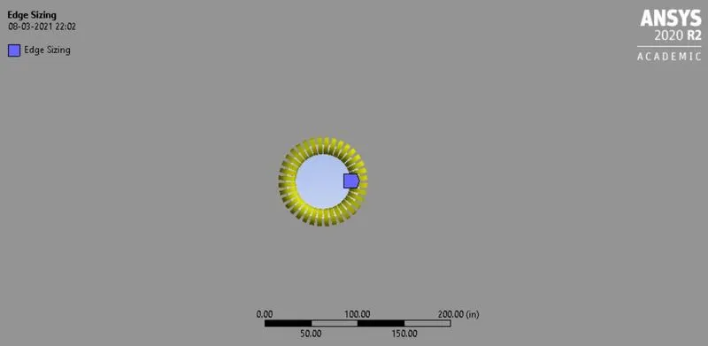
2. Edge sizing
It is carried out to make the circular region maintain its curved profile which will not be so when normal meshing is performed. Here, the curvature is divided into 36 divisions, which means that each element is spaced at 10deg.
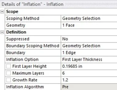
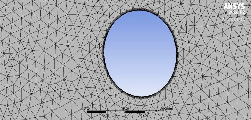
3. Inflation Layer
This stacks up multiple layers over the curved region in order to preserve the physics in boundary layer. Here, we have
Final Mesh:
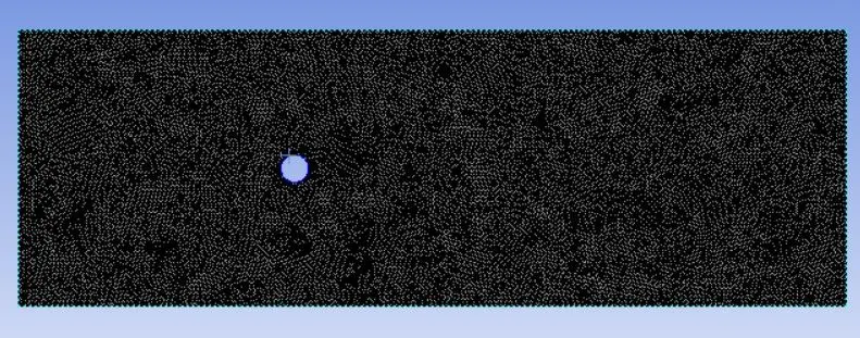
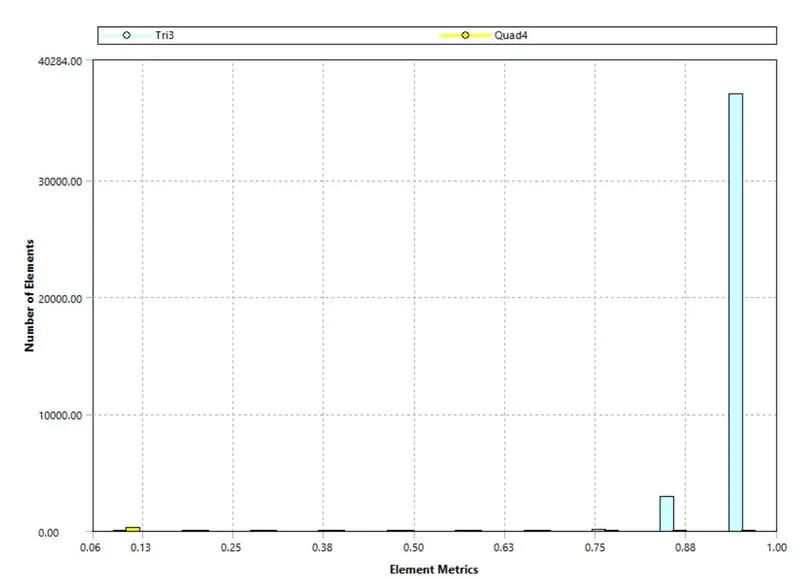
Here is the final mesh structure with 20696 nodes and 40500 elements. The quality of the mesh is also satisfactory as per the data from the histogram which shows majority of the elements are near to 1.

Named Selection:
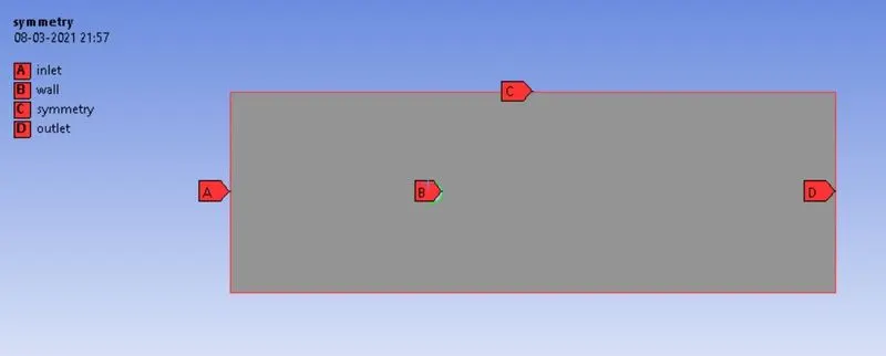
Named selections are user defined names such as inlet , outlet, wall for the cylinder and symmetry conditions for parallel edges between inlet and outlet. ANSYS detects automatically the type of boundary condistions to be defined based on the named selections defined by the user.
Case Setup: Case 1: Steady Case 2: Unsteady
1. Solver-Pressure based
2. Viscous model - Laminar
3. Working Fluid - air
Boundary Conditions: (velocity inlet,pressure outlet)
Initially, we set up Re = 100 as per our objective.
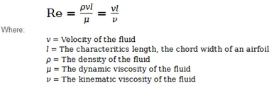
Density = 1 kg/m3
Viscosity = 0.02 kg/m-s
Characteristic length l = 2 m (Diameter of the cylinder)
Velocity inlet = 0.1 m/s
Pressure outlet = Gauge Pressure (0 Pa)
Iterations:
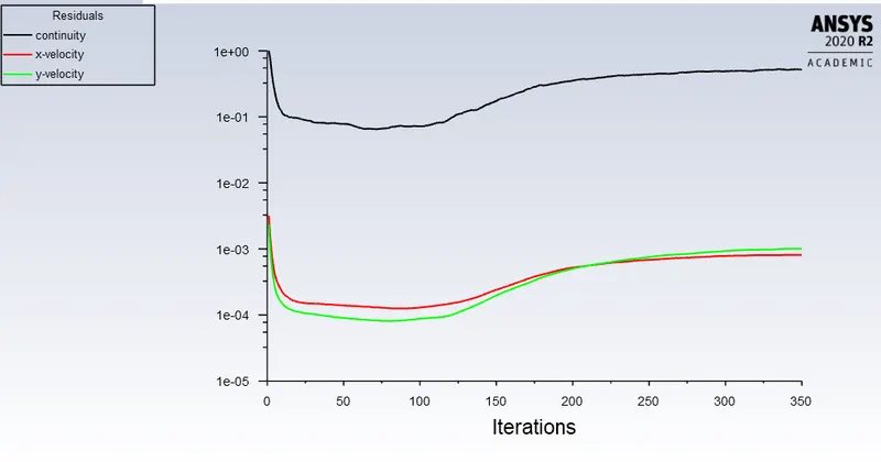
Steady: Simulation was set to run for 350 iterations.
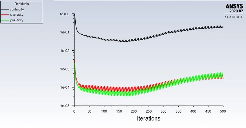
Unsteady:
Time step: 100
Time step size: 1 s
Max iterations/time step: 5
Total time: 100 s
Residual plot (Left:Steady, Right:Unsteady)
Convergence:
In steady state, the simulation runs for the set number of iterations unless any convergence criteria is specified under residual monitoring. Here, it was not set as the system may converge before vortex formation.
In transient/unsteady/time dependent case, for each time step, 5 iterations was performed. The repetitive fluctuation of x and y velocity shows that the flow is converging but not converged. This is due to the fact that the transient simulations are real time accurate. To get accurate convergence, the simulation has to be carried out for more time steps which requires computation and memory source. So the simulation was restricted with 500 iterations for 100 time steps.
Velocity contour: (Left:Steady, Right:Unsteady)
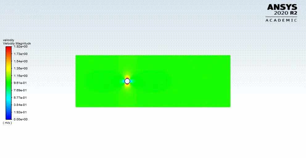
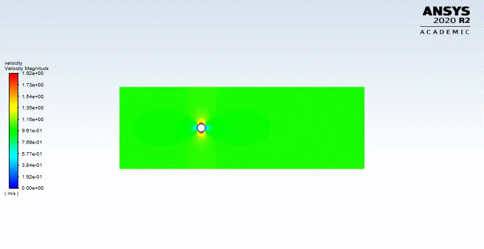
Pressure contour: (Left:Steady, Right:Unsteady)
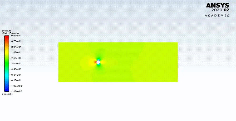
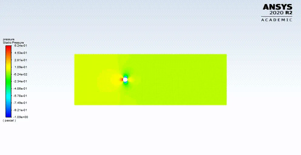
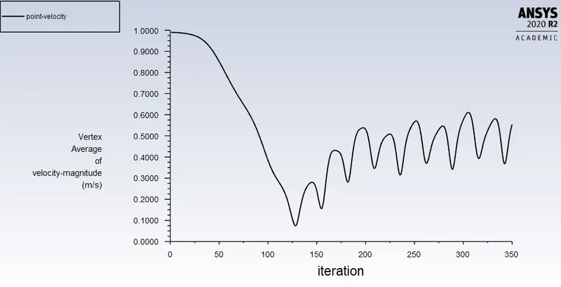
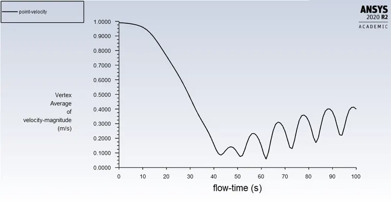
Vertex average of Velocity at (8,0): (Left:Steady, Right:Unsteady)
Strouhal Number:
The Strouhal Number is a dimensionless value useful for analyzing oscillating unsteady fluid flow dynamics problems.
The Strouhal Number can be expressed as
St = ω l / v
where, St = Strouhal Number, ω = oscillation frequency, l = characteristic length, v = flow velocity
The Strouhal Number represents a measure of the ratio of the inertial forces due to the unsteadiness of the flow or local acceleration to the inertial forces due to changes in velocity from one point to an other in the flow field.
Strouhal Number at (8,0):
Steady:
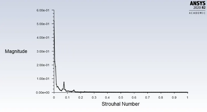
| Steady State | |
| Velocity m/s | Strouhal Number |
| 5.1952815e-01 | 0.0000000e+00 |
| 1.2299044e-03 | 9.9428570e-01 |
Unsteady:
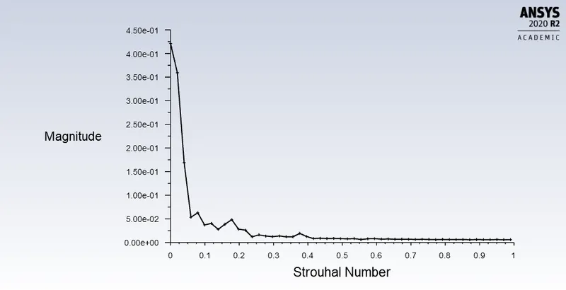
| Unsteady State | |
| Velocity m/s | Strouhal Number |
| 4.2100620e-01 | 0.0000000e+00 |
| 6.0403603e-03 | 9.9009901e-01 |
Inference: It can be seen that the strouhal number increases with decrease in velocity which is in corellation with the formula (inversely proportional).
PART II
Case Setup: Steady
1. Solver-Pressure based
2. Viscous model - Laminar
3. Working Fluid - air
4. Iterations - 350
v=0.5 m/s, Re=10
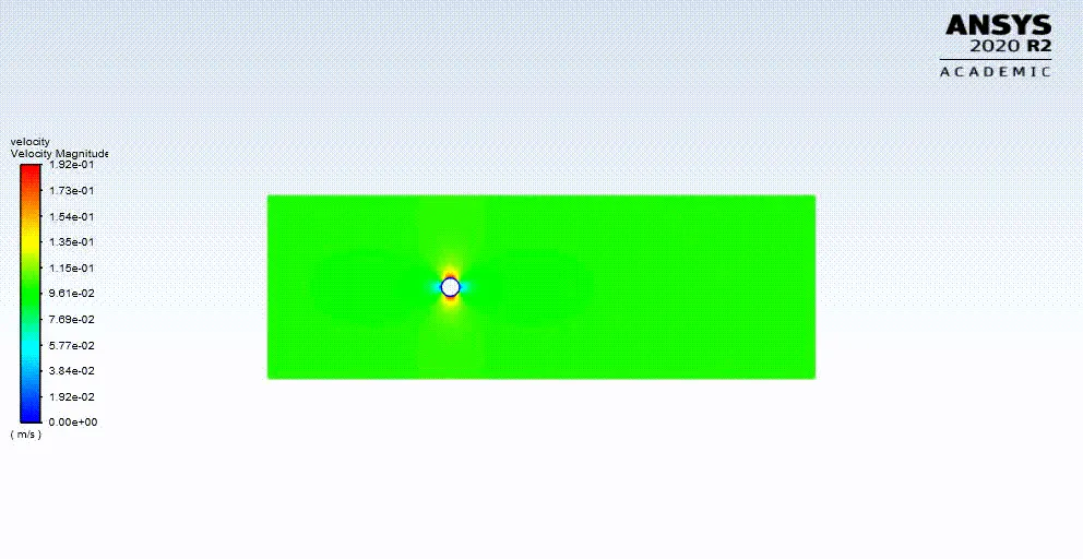
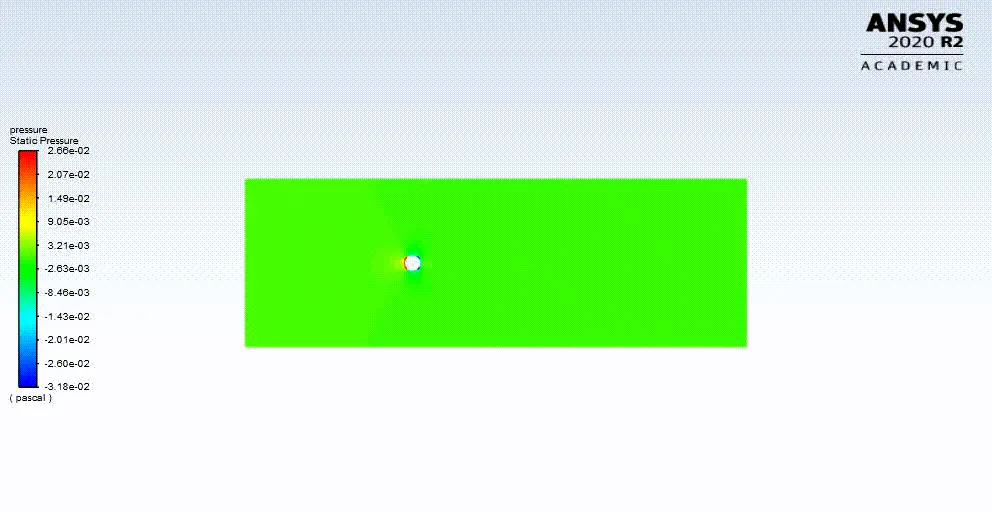
In above plots, vortex formation is not found as Re=10. Re has to be higher than 10 in order to visualise the vortex street formation.
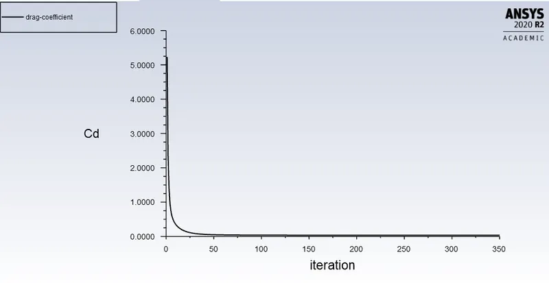
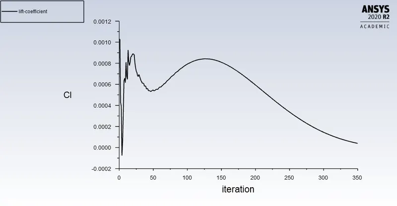
Above two plots, interpret the drag and lift coefficient at the cylindrical wall in the flow domain.
Drag Coeff. Cd=0.03349, Lift Coeff CL=3.99032e-05
v=1 m/s, Re=100
.
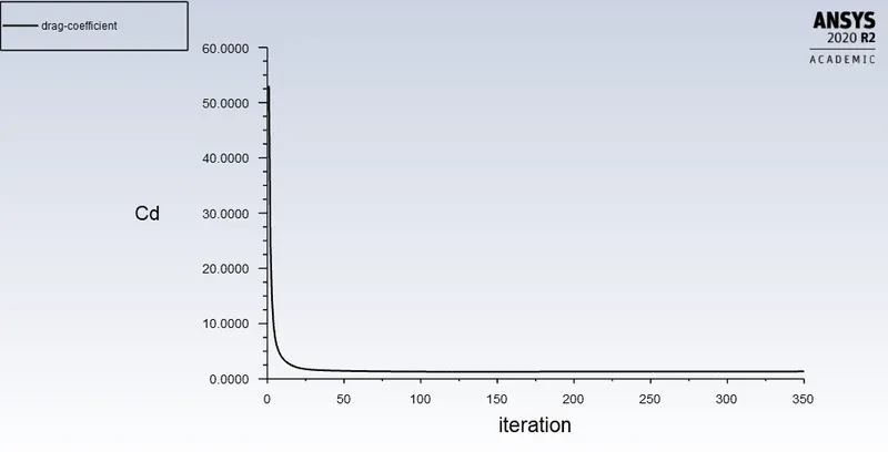
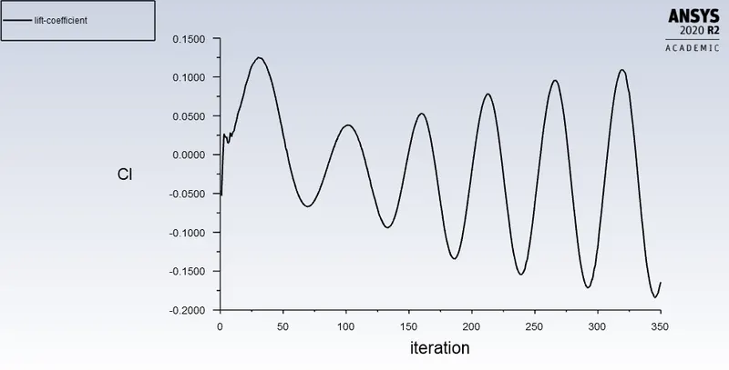
Drag Coeff. Cd=1.33760, Lift Coeff CL=-0.16409
v=10 m/s, Re=1000
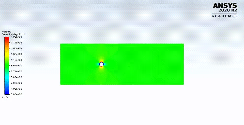
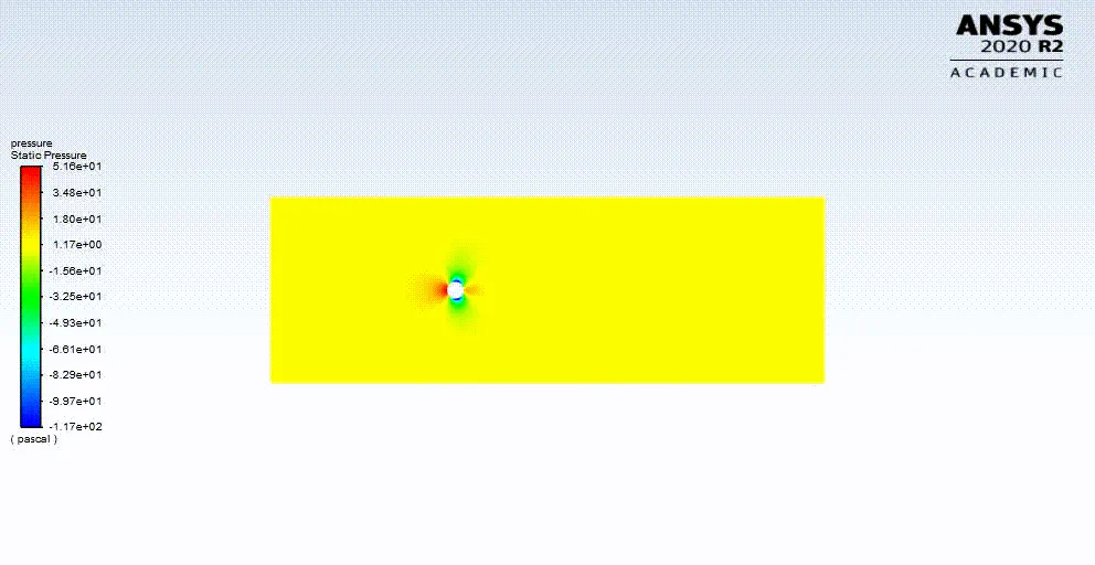
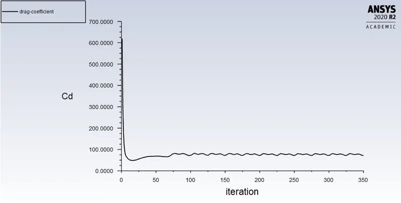
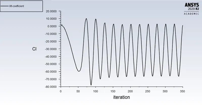
Drag Coeff. Cd=72.08378, Lift Coeff CL=-1.46033
v=100 m/s, Re=10000
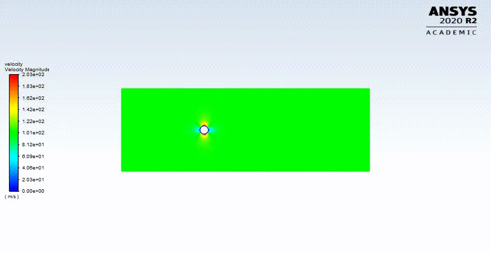
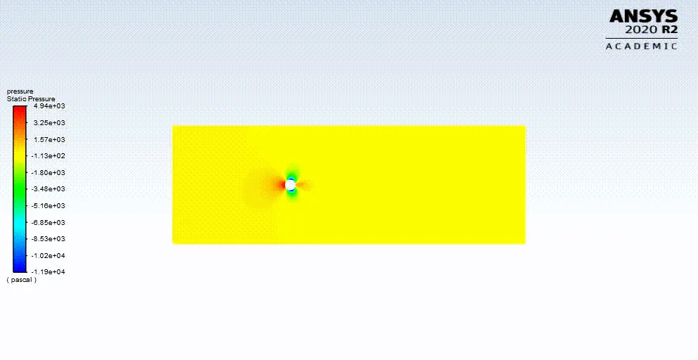
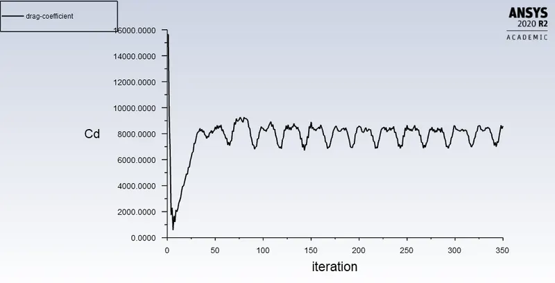
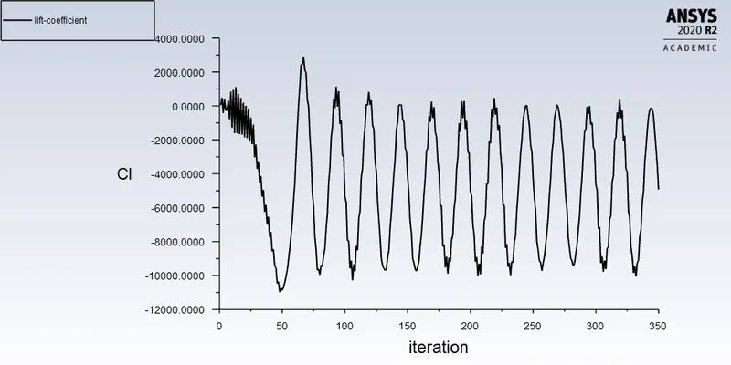
Drag Coeff. Cd=8582.55077, Lift Coeff CL=-4924.529472824525
v=1000 m/s, Re=100000
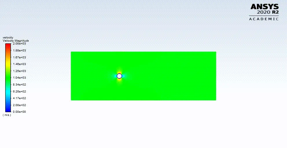
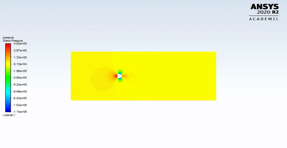
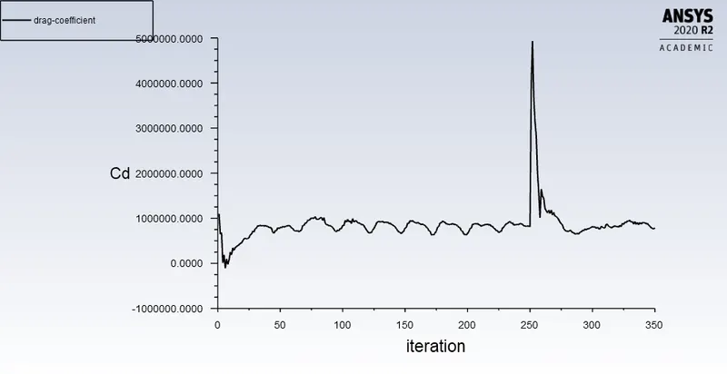
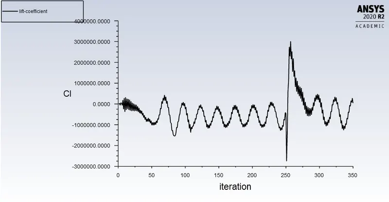
Drag Coeff. Cd=83229.54881, Lift Coeff CL=-109682.00430
Inference:
From the above plots, it is evident that the Drag Coeff increases with increasing Re, whereas Lift Coeff decreases with increasing Re.
Reference: https://www.sciencedirect.com/science/article/pii/S0307904X08000243