Week - 2 - Explicit and Implicit Analysis
Explicit and Implicit methods:
Explicit and implicit methods are approaches used in numerical analysis for obtaining numerical approximations to the solutions of time-dependent ordinary and partial differential equations, as is required in computer simulation of physical processes. Explicit methods calculate the state of a system at a later time from the state of the system at the current time, while implicit methods find a solution by solving an equation involving both the current state of the system and the later one. Mathematically, if Y(t) is the current system state and Y(t+dt)is the state at the later time (dt is a small-time step),
then, for an explicit method
Y(t+dt)=F(Y(t))
while for an implicit method one solves an equation
G(Y(t),Y(t+dt))=0 to find Y(t+dt)
"What are the consequences of using an implicit versus an explicit solution method for a time-dependent problem?"
1.The Stability Issue
The principal reason for using implicit solution methods, which are more complex to program and require more computational effort in each solution step, is to allow for large time-step sizes. A simple qualitative model will help to illustrate how this works. Let Q be a quantity whose value Qn+1 we want to compute at time t=(n+1)dt, in terms of its value at time t=ndt, i.e., Qn+1=Qn+dtS, where S is the rate of change in Q.
In an explicit numerical method, S would be evaluated in terms of known quantities at the previous time step n. An implicit method, in contrast, would evaluate some or all of the terms in S in terms of unknown quantities at the new time step n+1. Since new quantities then appear on both the left and right side of the Q-equation, it is said to be an implicit definition of the new n+1 values. Usually, a matrix or iterative solution must be used to compute the new quantities.
Numerical stability has to do with the behavior of the solution as the time-step dt is increased. If the solution remains well behaved for arbitrarily large values of the time step, the method is said to be unconditionally stable. This situation never occurs with explicit methods, which are always conditionally stable. It is easy to see that this is so by dividing the Q-equation by dt and then letting dt approach infinity. In this limit there are no n+1 terms remaining in the equation so no solution exists for Qn+1, indicating that there must be some limit on the size of the time step for there to be a solution.
In an implicit formulation, a solution for the unknowns at level n+1 may be obtained for any size time step. Of course, the solution for very large times may not be realistic unless the implicit formulation has been carefully constructed.
2.The Accuracy Issue
When dt is sufficiently small only one iteration is necessary for convergence, which leads to Qn+1=Qn+dt/(1+Cdt)Sn. This shows that the implicit formulation adds a smaller change to Q in a one-time step than would occur in an explicit method because of the under-relaxation factor A=1/(1+Cdt) that multiplies the time step.
Conclusion:
The choice of whether an implicit versus explicit method should be used ultimately depends on the goal of the computation. When time accuracy is important, explicit methods produce greater accuracy with less computational effort than implicit methods.
---------------------------------------------------------------------------------
Example: manually solving a physical problem whose force-displacement relation is given by `f(u)=u^3+9u^2+4u`
Now from the force-displacement equation
stiffness can be written as `k(u)=(df)/(du)=3u^2+18u+4`
1.explicit analysis:
Step1:
`u_0=0,Deltaf=1`
`k(u_0)=3(0)^2+18(0)+4=4`
`Deltau_1=(Deltaf)/(k(u_0))=1/4=0.25`
`u_1=u_0+Deltau_1=0+0.25=0.25`
`(F_(Internal))_1=f(u_1)=(0.25^3)+(9*0.25^2)+(4*0.25)=1.5781`
`(F_(external))_1=Deltaf=1`
Step2:
`u_1=0.25,Deltaf=1`
`k(u_1)=3(0.25)^2+18(0.25)+4=8.6875`
`Deltau_2=(Deltaf)/(k(u_1))=1/8.6875=0.1151`
`u_2=u_1+Deltau_1=0.25+0.1151=0.3651`
`(F_(Internal))_2=f(u_2)=(0.3651^3)+(9*0.3651^2)+(4*0.3651)=2.708`
`(F_(external))_2=Deltaf+Deltaf=2`
Step3: similarly u3 is calculated.
| Step i | the force applied in the step | change in displacement | total displacement | external force | internal force | residual = internal force-external force |
| 1 | 1 | 0.25 | 0.25 | 1 | 1.5781 | 0.5781 |
| 2 | 1 | 0.1151 | 0.3651 | 2 | 2.708 | 0.708 |
| 3 | 1 | 0.0911 | 0.4562 | 3 | 3.7928 | 0.7928 |
2.Implicit analysis
Step1:
`u_0=0,Deltaf=1`
`k(u_0)=3(0)^2+18(0)+4=4`
`Deltau_1=(Deltaf)/(k(u_0))=1/4=0.25`
`u_1=u_0+Deltau_1=0+0.25=0.25`
`(F_(Internal))_1=f(u_1)=(0.25^3)+(9*0.25^2)+(4*0.25)=1.5781`
`(F_(external))_1=Deltaf=1`
`Residual (R^0)=(F_(Internal))_1-(F_(enternal))_1=1.5781-1=0.5781`
`R^(0)>10^-2` so newton-raphson interations are necessary
calculating the correction-1
`deltau^1=-[k(u_1^0)]^-1*R^0=-(8.6875)^-1*0.5781=-0.0665`
updated value of u1 is
`u_1^1=u_1^0+deltau^1=0.25-0.065=0.1835`
checking residual again
`(F_(Internal))_1=f(u_1)=(0.1835^3)+(9*0.1835^2)+(4*0.1835)=1.0432`
`Residual (R^1)=(F_(Internal))_1-(F_(enternal))_1=1.0432-1=0.0432`
`R^(1)>10^-2` so newton-raphson interations are necessary
calculating the correction-2
`deltau^2=-[k(u_1^1)]^-1*R^1=-(7.404)^-1*0.0432=-0.005835`
updated value of u1 is
`u_1^2=u_1^1+deltau^2=0.1835-0.005835=0.1777`
checking residual again
`(F_(Internal))_1=f(u_1^2)=(0.1777^3)+(9*0.1777^2)+(4*0.1777)=1.0006`
`Residual (R^0)=(F_(Internal))_1-(F_(enternal))_1=1.0006-1=0.0006`
`R^(0)<10^-2` so newton-raphson interations are not necessary necessary
so
`t the end of the step1, u_1=u_1^2=0.1777`
similarly, step 2 and step3 are done.
| Step i | the force applied in the step | total displacement | external force | internal force | residual = internal force-external force |
| 1 | 1 | 0.1777 | 1 | 1.0006 | 0.0006 |
| 2 | 1 | 0.2966 | 2 | 2.0042 | 0.0042 |
| 3 | 1 | 0.3911 | 3 | 3.0008 | 0.0008 |
comparison:
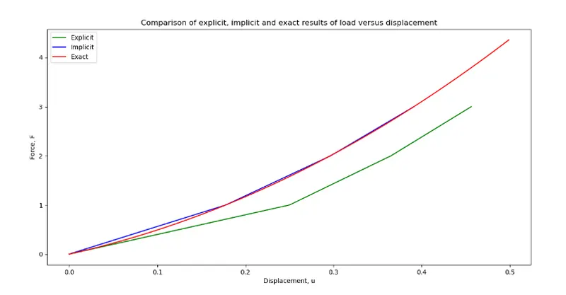
Conclusion:
It is evident from the results that the explicit analysis
drifts from the true solution. To overcome this problem an implicit analysis is used, which
includes Newton-Raphson iterations to enforce equilibrium between internal and external
forces.
By increasing the no of steps(reducing timestep), explicit analysis results can be more accurate but it requires more time.