Week - 2 - Explicit and Implicit Analysis
Objective:
- To solve the given equation with both the explicit and implicit methods and plot the graphs of Force v/s Displacement for the methods.
Introduction:
- Explicit and Implicit methods are two different types to approach any Ordinary Differential Equations (ODE) and Partial Differential Equations (PDE), which numerically denotes the computer simulations.
- Explicit method uses all the terms from the previous timestep to compute or to determine the current timestep. While, on the other hand, the Implicit method uses the displacement from the previous timestep and expresses force as a function. The implicit method demands the need of matrix inversion.
- But these two methods are two different schemes altogether to solve the same problem. The explicit method assumes the convergence for all the time step and doesn't check for the same after every timestep. On the other hand, the implicit method checks the convergence after every timestep before proceeding further.
- This makes the results more accurate but on the other hand, increases the computation or the calculation time for the implicit method when the equation is more of a complex nature. This is because several iterations are needed to perform in order to reach the convergence. The explicit method, since does not check for convergence after every timestep, takes lesser time for computation, but it also has problems with stability.
- To avoid this, the timesteps in the explicit methods have to be kept very small, and in most cases, the user does not have control over the selection of these extremely small timesteps. On the other hand, in the implicit method, the user can control the size of the timesteps.
Problem:
- The equation that has to be solved is as followed:
`F(u)=(u)^3+9(u)^2+4(u)`
- Here, we will consider the following notations for force and displacement:
`F=External Force`
`DeltaF=Incremental Force`
`u= Displacement`
`Deltau= Incremental Displacement`
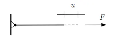
- Let us consider a simple bar in tension as shown in the image. The force on the free end of the bar can be considered as a non-linear function of displacement in the form of the equation given above.
- Then the stiffness of the bar can be computed as
`k(u)=d/(du) F(u)`
`d/(du)F(u)=3u^2+18u+4`
Explicit Method:
- Displacement=Force/Stiffness=`F/k`
- Let the initial condition be `DeltaF=1`
- Displacement,
`u_(i+1)= u_i +du_i` - Step 1:
Let `u(0)=0`, then
`k(u_0)=3(0)^2+18(0)+4 =4`
`Deltau_1=(DeltaF)/k =1/4 = 0.25`
`u_1=u(0)+Deltau_1`
`=0+0.25 =0.25`
`F(u_1)=(0.25)^3+9(0.25)^2+4(0.25)=1.578` - Step 2:
Let `u=u_1 =0.25`
`k(u_1)=3(0.25)^2+18(0.25)+4 =8.687`
`Deltau_2=(DeltaF)/k=1/8.687=0.115`
`u_2=u_1+Deltau_2=0.25+0.115=0.365`
`F(u_1)=(0.365)^3+9(0.365)^2+4(0.365)=2.709` - Step 3:
Let `u=u_2=0.365`
`k(u_2)=3(0.365)^2+18(0.365)+4 =10.96`
`Deltau_3=(DeltaF)/k=1/10.96=0.091`
`u_3=u_2+Deltau_3 =0.365+0.091=0.456`
`F(u_3)=(0.456)^3+9(0.456)^2+4(0.456)=3.793` - `F_(ext)=Delta F+Delta F+Delta F =1+1+1=3`
-
Steps `DeltaF` `Delta u` `u` `F_(ext)` `F_i` `F=F_i-F_(ext)` 0 0 0 0 0 0 0 1 1 0.25 0.25 1 1.578 0.578 2 1 0.115 0.365 2 2.707 0.707 3 1 0.091 0.456 3 3.791 0.791
Implicit method:
- The explicit method assumes equilibrium to exist at all times and directly moves forward to calculate the variables. On the other hand, the implicit method checks for convergence after every timestep and then only move forward for the calculation of the variables. This convergence is brought by using the Newton-Raphson method with its iterations. For convergence `F_(ext)`should be equal to `F`or the residual `R=F-F_(ext)=0`. After each timestep, the residual needs to be brought within the tolerance value. Here the tolerance value that we are assuming is 0.01. This is done by using the Newton-Raphson iteration to calculate the correction values until the required tolerance value is reached.
- The residual R can be expanded in the form of the Taylor series about the current displacement `u_j`, which gives,
`R^(j+1)=R^j(u^j)+(dR(u^j))/(du)deltau^(j+1)+...`
`=R^j+k(u^j)deltau^(j+1)+...`
By neglecting the higher-order terms in the series and setting `R^(j+1)=0`, and solving for `deltau^(j+1)`, we get following correction:
`deltau^(j+1)=-[k(u_j)]^-1R^j`
Here the iteration variable is `j`and it may take several iterations for the normal residual `||R||`to reach within the tolerance value.
Now we can solve using the implicit method as follows: - Force function, `F(u)= (u)^3+9(u)^2+4(u)`
just like the previous steps, by differentiating the force function about `u`, we get the stiffness function so,
`k(u)=d/(du)F(u)=3(u)^2+18(u)+4`
Displacement, `u=F/k`
Force increment, `DeltaF=1`
Displacement increment, `Delta u=(DeltaF)/k`
Displacement, `u_(i+1)=u_i+Deltau_(i+1)` - Step1:
Let `u=0`
`k(0)=9(0)^2+18(0)+4=4`
`Deltau_1=(DeltaF)/(k(u_0))=1/4=0.25`
`u_1=u_0+Deltau_1=0+0.25=0.25`
`F(u_1)=(u_1)^3+9(u_1)^2+4(u_1)=(0.25)^3+9(0.25)^2+4(0.25)=1.578`
`F_(ext)=1`
Therefore the Residual R becomes, `R^0=F_1-F_(ext)=1.578-1=0.578`
But since `||R||>0.01`, we have to solve further using the Newton-Raphson iterations, which would bring R closer to the tolerance value. - Iteration 1:
Let `u_1^0=u_1=0.25`
Correction factor for `u_1=delta(u_1)^1=-[k(u_1^0)]^-1R^0`
`k(u_1^0)=k(u_1)=3(0.25)^2+18(0.25)+4=8.688`
Therefore, `delta(u_1)^1=-[k(u_1^0)]^-1R^0=-(8.688)^-1(0.578)=-0.06653`
Corrected `u_1=u_1^1+deltau_1^1=0.25+(-0.06653)=0.183`
Updated residual `R^1=F^(1)-F_(ext)`
`F^((1))=(u_1^((1)))^3+9(u_1^((1)))^2+4(u_1^((1)))=(0.183)^3+9(0.183)^2+4(0.183)=1.039`
`R^1=1.039-1=0.039`
Again `||R||>0.01` Therefore, proceed to second iteration. - Iteration 2:
Correction factor for `u_1=deltau_1^((2))=deltau_1-[k(u_1^((1)))]^-1R^((1))`
`k(u_1^((1)))=3(0.183)^2+18(0.183)+4=7.394`
`delta u_1^((2))=(-0.06653)-(7.394)^-1(0.039)=0.1782`
Updated Residual `R^((2))=F^((2))-F_(ext)`
`F^((2))=(u_1^((2)))^3+9(u_1^((2)))^2+4(u_1^((2)))`
`=(0.1782)^3+9(0.1782)^2+4(0.1782)=1.004`
`R^((2))=1.004-1=0.004`
Since, `||R||=0.004<0.01`, R is within the tolerance and there is no need for further iterations.
Therefore, `F(u_1)=F(u_1^((2)))=1.004`
and final correction value of `u_1=u_1^((2))=0.1782` - Step 2:
`DeltaF=1`
`k(u_1)=3(u_1)^2+18(u_1)+4=3(0.1782)^2+18(0.1782)+4=7.302`
`Deltau_2=(DeltaF)/(k(u_1))=1/7.302=0.137`
`u_2=u_1+Deltau_2=0.1782+0.137=0.315`
`F(u_2)=(u_2)^3+9(u_2)^2+4(u_2)`
`=(0.315)^3+9(0.315)^2+4(0.315)=2.184`
`F_(ext)=DeltaF+DeltaF=1+1=2`
`R=F(u_2)-F_(ext)=2.184-2=0.184`
`||R||>0.01`, therefore solve further using Netwon-Raphson iterations. - Iteration 1:
Let `u_2^((0))=u_2=0.315`
Correction factor for `u_2=deltau_2^((1))=-[k(u_2^((0)))]^-1R^0`
`k(u_2^((0)))=3(u_2^((0)))^2+18(u_2^((0)))+4=9.967`
and from above `R^((0))=0.184`
`deltau_2^((1))=-(9.967)^-1(0.184)=-0.0185`
Corrected `u_2=u_2^((1))=u_2+deltau_2^((1))`
`=0.315+(-0.0185)=0.296`
Updated Residual, `R^((1))=F^((1))-F_(ext)`
`F^((1))=(u_2^((1)))^3+9(u_2^((1)))^2+4(u_2^((1)))`
`=(0.296)^3+9(0.296)^2+4(0.296)=1.998`
`R^((1))=1.998-2=-0.002`
Therefore, `||R||=0.002<0.01`, which is within tolerance limit and there is no need of further iterations.
Hence, `F(u_2)=F(u_2^((1)))=1.998`
and final corrected value of `u_2=u_2^((1))=0.296 - Step 3:
`DeltaF=1`
`k(u_2)=3(u_2)^2+18(u_2)+4`
`=3(0.296)^2+18(0.296)+4=9.59`
`Deltau_3=(DeltaF)/(k(u_2))=1/9.59=0.104`
`u_3=u_2+Deltau_3=0.296+0.104=0.4`
`F(u_3)=(u_3)^3+9(u_3)^2+4(u_3)`
`=(0.4)^3+9(0.4)^2+4(0.4)=3.104`
`F_(ext)=DeltaF+DeltaF+DeltaF=1+1+1=3`
`R=F(u_3)-F_(ext)=3.104-3=0.104`
`||R||>0.01`, therefore solve further using Netwon-Raphson iterations. - Iteration 1:
Let `u_3^((0))=u_3=0.4`
Correction factor for `u_3=deltau_3^((1))=-[k(u_3^((0)))]^-1R^0`
`k(u_3^((0)))=3(u_3^((0)))^2+18(u_3^((0)))+4`
`=3(0.4)^2+18(0.4)+4=11.68`
and from above, `R^((0))=0.104`
`deltau_3^((1))=-(11.68)^-1(0.104)=-0.0089`
Corrected `u_3=u_3^((1))=u_3+deltau_3^((1))`
`=0.4+(-0.0089)=0.3911`
Updated Residual, `R^((1))=F^((1))-F_(ext)`
`F(u_3)=(u_3^((1)))^3+9(u_3^((1)))^2+4(u_3^((1)))`
`=(0.3911)^3+9(0.3911)^2+4(0.3911)=3.008`
`R^((1))=3.008-3=0.008`
`||R||<0.01` which is within the tolerance limit and there is no need for further iterations.
Therefore, `F(u_3)=F(u_3^((1)))=3.008`,
and final corrected value of `u_3=u_3^((1))=0.3911` -
Steps `DeltaF` `Deltau` `F_(ext)` `F_i` `R=F_i-F_(ext)` `u_i` Corrected `u_i` 0 0 0 0 0 0 0 1 1 0.25 0.178 1 1.004 0.004 2 1 0.365 0.296 2 1.998 -0.002 3 1 0.456 0.391 3 3.008 0.008
Result and Conclusion:
- Graphs of Force v/s Displacement of the solutions from both the Implicit and Explicit analyses were plotted in Excel as seen in the image below. This is done to visualize the difference between the results of the Implicit and Explicit methods for the same force function.
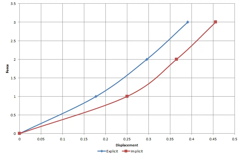
- It can be observed that the explicit solutions are deviating as more and more load is being applied. If the graph for the exact solution is plotted, it will perfectly overlap with implicit solution. The Newton-Raphson method has corrected the incremental steps so that they land on the exact solution according to specified tolerance.
- The Newton-Raphson iterations are used to enforce equilibrium before moving towards the next step. In implicit method, incremental force is applied to advance to the solution forward. These internal and external forces are not in equilibrium and hence the displacement should be controlled for equilibrium. This is done by Newton-Raphson iterations to minimize the residual.