Explicit and Implicit Analysis

Implicit Analysis:

The meaning of implicit is that it can't be discriminate(separated).

suppose we have an equation: `x^y=e^(xy)+x`

to solve this equation we need to do it with some iterative method therefore it can't be solved directly. so we need to take some initial values as x and then we need to try to converge the solution.

`[M][ddotX]+[C][dotX]+K[X]= F`

`[X]=[K]^-1{{F}-[M][ddotX]+ C[dotX]}`

where k^-1 is the inverse of stiffness matrix

therefore `{D}_(n+1)= f({ddotD}_(n+1),{ddotD}_n,{D}_n,{dotD}_n....)`

Explicit Analysis:

The meaning of implicit is that it can be discriminate

suppose we have an equation: `x=e^(xy)-> ln(x)=xy-> y=lnx/x`

`[M][ddotX]+[C][dotX]+K[X]= F`

`[ddotX]=M^-1({f}-[C][dotX]+K[X])`

where M^-1 is the mass inversion matrix.

therefore `{D}_(n+1)= f({D}_(n),{ddotD}_n,{D}_n,{dotD}_n....)`

Differences[ Implicit vs Explicit]

Implicit	Explicit
In the implicit scheme, unknown X find by inversion of stiffness matrix[k]	In an Explicit analysis scheme, the unknown can be found by inversion of mass matix[M]
For each increment The stiffness matrix is updated Next increment load defined Newton-Rapson enforce equilibrium	For each increment The stiffness matrix is updated Next increment load defined Direct solution
we use the Newmark-β method (numerical integration method)	we use the central difference method
unconditionally stable for any initial assumption of △t solution converges	conditionally stable we need to take of critical time step value △t<△tcr
More Accurate	Less Accurate
Extremely time-consuming for large model	computationally efficient for the larger models with relatively short dynamic response time.
No mathematically time limit for the solution	Time taken depends on the wave propagation speed & characteristic length of the element
Implicit require much more computer storage	Less storage required than an implicit method

When to use Implicit and Explicit?

strain rates/velocity is lower, say less than 10units/sec	strain rates/velocity is higher, say more than 10units/sec
Effects of strain rates are minimum	strain rates have a significant effect.
Easy or moderate contact condition.	Can solve complex contact condition
Growth of stress is a function of strain and once this established these can be analyzed using implicit method	Variation of stress is a function of strain but also strain rate.

Application

Good choice for structural dynamics type problem for which load rates are slow such as, low-frequency response Vibration Oscillation

best suited for wave propagation type of problem with high strain rates. Car crash Drop Impact Blast etc.

PROBLEM

Equation: `u^3+9u^2+4u`

`f(u)/(du)=K(u)= 3u^2+18u+4`

(stiffness of the rod)

`triangleF=1` External force step

#Explicit Analysis#

`triangle U=(triangle F)/(K(u))`

step1:

`u_0=0, K(u_0)=4, triangleF=1, triangleU_1=(triangleF)/(K(u))=1/4`

therfore `triangleU_1=0.25 -> u_1-u_0= 0.25-> u_1=0.25 mm`

step2:

`u_1=0.25, K(u_1)=8.687, triangleF=1, triangleU_2=(triangleF)/(K(u_1))=1/8.687`

therfore `triangleU_2=1/8.687 -> u_2-u_1=1/8.687 -> u_2=0.3651 mm`

step3:

`u_2=0.3651, K(u_2)=10.96, triangleF=1, triangleU_3=(triangleF)/(K(u_2))=1/10.96`

therfore `triangleU_3=1/10.96 -> u_3-u_2=1/10.96 -> u_3=0.456 mm`

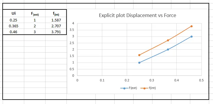
`F_(ext)= triangleF+triangleF+triangleF= 3`

`f_(Int)=u^3+9u^2+4u= 3.791`

Results are evident that external and internal forces are not in equillibrium `F_(ext)!= F_(Int)`

#Implicit Method#

Step-[1]

`U_0=0, K(U_0)=4, triangle F=1, triangleU_1=1/4=0.25`

`U_1-U_0=0.25, U_1=0.25`

check the residual `-> F_(ext)=triangleF= 1`

`f_(Int )= u^3+9u^2+4u`

`f_(Int)= 1.578`

`R=1.578-1=|0.578|> 10^(-2)`

N-R Iteration [1]

`delu^1=[K(u_i)]^-1 *R^0= -0587/8.687= -0.0665`

`delu^1=0.0665-> u_1= 0.25-0.0665= 0.1834`

Check for residual:

`f_((0.1834))= 1.0424`

`R=1.0424-1=|0.0424|> 10^(-2)`

Iteration No.[2]

`delu^2=[K(u_1)]^-1 *R^1= -0.0424/7.402 = -0.00572`

`u_1^2= 0.1834-0.00572= 0.1776`

`f(0.1776)=0.9998`

`R= |0.9998-1|=0.0002<10^-2`

well satisfied

Step-[2]

`U_1=0.1776, K(U_1)=7.29 , triangle F=1, triangleU_2=1/7.29`

`U_2-U_1=0.1371, U_2=0.3147`

`f_((0.3147))= 2.1743`

`R=2.1743-2=|0.1743|> 10^(-2)`

N-R iteration

`delu=-(0.1743)/9.963= -0.0174`

`U_2^1-U_2=-0.0174, U_2= 0.2965`

`f_((0.2965))= 2.0006`

`R=2.0006-2=|0.0006|<10^(-2)`

Satisfied

Step-[3]

`U_2=0.2965, K(U_2)=9.6008 , triangle F=1, triangleU_3=1/9.6008`

`U_3-U_2=0.01041 -> U_3=0.4006`

`f_((0.4006))= 3.111`

`R=3.111-3=|0.111|>10^(-2)`

N-R iteration

`delu=-(0.111)/11.69= -0.0094`

`u_3^'= 0.3911`

`f(0.3911)= 3.0085`

`R=3.0085-3=|0.0085|<10^(-2)`

satisfied

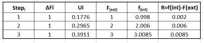
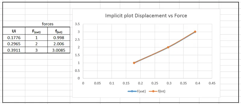
Results are evident that external and internal forces are in equilibrium `F_(ext)-= F_(Int)`