Week - 2 - Explicit and Implicit Analysis

Aim:

To give detailed report about Explicit and Implicit methods and to solve F(u)=u³+9u²+4u using both Explicit and Implicit methods (with a tolerance of 10^-2)

Explicit and Implicit Method:

Implicit and Explicit analysis differ in the approach to time incrementation. In Implicit analysis each time increment has to converge, but you can set pretty long time increments. Explicit on the other hand doesn’t have to converge each increment, but for the solution to be accurate time increments must be super small.

You will use Implicit and Explicit solvers to solve dynamic problems. This means that you won’t need to know this stuff if you are doing static analysis.

Dynamic analysis solves problems involving inertia effects. Those appear, when things change fast in your model (quickly applied loads, impacts, etc.). Engineers usually reffer to this as “nonlinear dynamic”.

It should be noted, that often engineers call other analysis “dynamic” as well. Things like Modal analysis or Forced Response analysis that deal with vibrations. Sometimes those are called “linear dynamic”, but it is usually a good idea to make sure what someone means when they use such a phrase.

The first thing I really feel I have to stress is that implicit and explicit solvers solve THE SAME problems! Think about it not as “different solvers” but rather as two different ways of solving the same problem.

In many cases, you can use both implicit and explicit solver, and they will produce the same outcome.

How Implicit Analysis Works:

First of all, implicit seems to be a more “basic” solution. In essence it works just as you would think it should!

Firstly, in each time increment the “global equilibrium” in the model is established. This means that each increment has to converge (this is happening in iterations).

After global equilibrium is ok, solver calculates all the local finite element variables (stresses etc.) for this increment.

Benefits: Since global equilibrium is verified at each time increments, those increments can be BIG!

Drawbacks: Each time increment computes slowly, since iterations are needed to get to the global equilibrium.

How Explicit Analysis Works:

This one is funky. It works in a way, that you don’t have to converge each step! There are no convergence criteria to check and… no iterations! Instead of verifying the “global equilibrium” solver assumes that the equilibrium “simply exists”. This means that the solver goes straight into calculation of local finite element variables! As such procedure has only one step:

Calculate all of the local finite element variables for given increment, and move to the next one!

Benefits: Each increment calculates extremely fast!

Drawbacks: For this to work, the time step has to be EXTREMELY small. Otherwise, it’s impossible to maintain this equilibrium that is assumed to “simply exist”. To achieve this, user do not have direct control over how big-time increments explicit solver will take. Solver itself calculates how small timesteps are still ok. And those acceptable time increments are SUPER SMALL! This is why explicit problems should last fractions of the second! If they would last seconds… you would need millions of increments!

The Excel Sheet attached with the assignment calculates the equation

F(u)=u³+9u²+4u

using both Explicit and Implicit methods (with a tolerance of 10^-2).

In both methods, Delta F =1 is added after each step.

In Explicit method, Delta U is calculated by

Delta U = Delta F/K_u

Where K_u is the stiffness at displacement u.

Then subsequent displacements are calculated using

U₂=U₁+Delta U

Corresponding F is calculated.

In Implicit method,

F is calculated in the same way but is compared with the original value.

Residue=F_internal-F_external

If Residue is greater than a fixed tolerance value, Delta U is recalculated using

Delta U^j+1 = -[k(u^j)]^-1R^j

Where j is the iteration variable

R is the Residue

This delta U is added to the original displacement U and corresponding F is calculated.

Iteration continues till Residue is less than the tolerance value

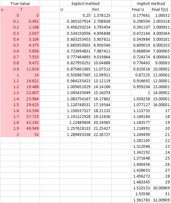
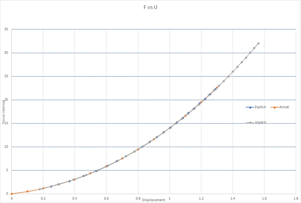
Since the incremental Force is very less, both implicit and explicit analysis almost matches with the exact solution.