Week - 2 - Explicit and Implicit Analysis
OBJECTIVE :
To solve the provided equation using both Explicit and Implicit Methods
THE PROBLEM :
Consider the case of a simple bar in tension, suppose that the force in the bar is a nonlinear function of the displacement, solve the function using mentioned methods.
`F(u) = u^3 + 9u^2 + 4u`
By differentiating the above force equation w.r.t. displacement "u", we can get the equation of stifness.
`k(u) = (dF)/dt = 3u^2 + 18u + 4`
THEORY :
What is Explicit Analysis :
Explicit analyses aim to solve for acceleration (or otherwise {x´´}). In most cases, the mass matrix is considered as “lumped” and thus a diagonal matrix. Inversion of a diagonal matrix is straightforward and includes inversion of the terms on the diagonal only. Once the accelerations are calculated at the nth step, the velocity at n+1/2 step and displacement at n+1 step are calculated accordingly. In these calculations, the scheme is not unconditionally stable and thus smaller time steps are required. To be more precise, the time step in an explicit finite element analysis must be less than the Courant Time step (i.e., the time taken by a sound wave to travel across an element).
What is Implicit Analysis :
One method of solving for the unknowns {x} is through matrix inversion (or equivalent processes). This is known as an implicit analysis. When the problem is nonlinear, the solution is obtained in a number of steps and the solution for the current step is based on the solution from the previous step. For large models, inverting the matrix is highly expensive and will require advanced iterative solvers (over standard direct solvers). Sometimes, this is also known as the backward Euler Integration Scheme. These solutions are unconditionally stable and facilitate larger time steps. Despite this advantage, the implicit methods can be extremely time-consuming when solving dynamic and nonlinear problems.
Difference Between Implicit and Explicit Analysis :
Explicit FEM is used to calculate the state of a given system at a different time from the current time. In contrast, an implicit analysis finds a solution by solving an equation that includes both the current and later states of the given system. This method requires additional computation and can be harder to implement. However, it will be used in lieu of explicit methodologies when problems are still and using alternative analysis methods is impractical.
SOLUTION :
Exact Value :
We know that the value of Force at each step increases by 1 unit. Therefore by substituting the value in the force equation provided and solving for displacement we get.
STEP 1 :
F = 1;
`1 = u^3 + 9u^2 + 4u`
u = 0.178
STEP 2 :
F = 2;
`2 = u^3 + 9u^2 + 4u`
u = 0.296
STEP 3 :
F = 3;
`3 = u^3 + 9u^2 + 4u`
u = 0.391
| STEP | Force | Displacement |
| 0 | 0 | 0 |
| 1 | 1 | 0.178 |
| 2 | 2 | 0.296 |
| 3 | 3 | 0.391 |
Explicit Analysis :
Clearly it is possible to plot a graph of force, f, versus displacement, u, by using the above equations, However, if the nonlinear force versus displacement relationship is not known, but the stiffness is known, it is possible to construct the graph of force versus displacement numerically. One method is to use an incremental explicit load control scheme.
This is illustrated next. For this example three equal load increments (or steps) of ∆F = 1unit each are used to load the tension bar. The variables used are
u for displacement
f for internal force in the bar
F for external force applied to the bar (and)
k for stiffness.
Incremental displacements or incremental externally applied forces are represented as ∆u or ∆F respectively. Use is made of the relationship ∆F = k∆u. The analysis proceeds as follows.
We know that,
Equation of force : `F(u) = u^3 + 9u^2 + 4u`
Stiffness Equation : `k(u) = 3u^2 + 18u + 4`
Displacement increment = `Delta u_i = (dF)/K`
Displacement = `u_(i+1) = u_i + Delta u_(i+1)`
Assuming Load Step increment dF = 1,
Step - 1 :
`u_0 = 0`,
`F(u_0) = 0`
`k(u_0) = 3*(0)^2 + 18*(0) + 4 = 4`
`Deltau_1 = (dF)/(k(u_0)) = 1/4 = 0.25`
`u_1 = u_0 + Deltau_1 = 0 + 0.25 = 0.25`
`F(u_1) = (0.25)^3 + 9*(0.25)^2 + 4(0.25) = 1.578`
`F_(ext-1) = dF = 1`
Step - 2 :
`u_1 = 0.25`,
`k(u_1) = 3*(0.25)^2 + 18*(0.25) + 4 = 8.6875`
`Deltau_2 = (dF)/(k(u_1)) = 1/8.6875 = 0.115`
`u_2 = u_1 + Deltau_2 = 0.25 + 0.115 = 0.365`
`F(u_2) = (0.365)^3 + 9*(0.365)^2 + 4(0.365) = 2.709`
`F_(ext-2) = dF+dF = 2`
Step - 3 :
`u_2 = 0.365`
`k(u_2) = 3*(0.365)^2 + 18*(0.365) + 4 = 10.972`
`Deltau_3 = (dF)/(k(u_2)) = 1/10.972 = 0.091`
`u_3 = u_2 + Deltau_3 = 0.365 + 0.091 = 0.456`
`F(u_3) = (0.456)^3 + 9*(0.456)^2 + 4(0.456) = 3.793`
`F_(ext-3) = dF+dF+dF = 3`
| Step | `(dF)_i` | `Deltau_i` | `u_i` | `(F_(ext))_i` | `(f_(Int))_i` | `f_(Int) - F_(ext) = R` |
| 0 | 0 | 0 | 0 | 0 | 0 | 0 |
| 1 | 1 | 0.25 | 0.25 | 1 | 1.578 | 0.578 |
| 2 | 1 | 0.115 | 0.365 | 2 | 2.709 | 0.709 |
| 3 | 1 | 0.091 | 0.456 | 3 | 3.793 | 0.793 |
Implicit Analysis :
An implicit analysis is the same as the explicit analysis, except that at the end of each step Newton-Raphson iterations are used to enforce equilibrium before moving to the next step. Basically, an incremental force is applied to advance the solution forward at the beginning of a step. However, internal forces and external forces will not be in equilibrium unless the stiffness is linear for the given step.
Hence, in order to achieve equilibrium, corrections must be made to the displacement. This is accomplished by using Newton-Raphson iterations to minimize the residual,
R(u) = fint − Fext.
Expanding the residual as a Taylor series about the current displacement u gives,
`R^(j+1) = R^j(u^j) + (dR(u^j))/(du) deltau^(j+1) + .... = R^j + k(u^j)deltau^(j+1) + ...`
By neglecting higher order terms in the series, setting `R^(j+1) = 0`and solving for `deltau^(j+1)` the following correction is obtained
`deltau^(j+1) = -[k(u^j)]^-1R^j`
Notice that the iteration variable is j and it may take several iterations for the norm of the residual, `norm(R)`, to be reduced below the chosen tolerance criteria (in this case, below a tolerance of 10−2). The implicit analysis proceeds as follows.
Step - 1 :
`u_0 = 0`,
`F(u_0) = 0`
`k(u_0) = 3*(0)^2 + 18*(0) + 4 = 4`
`Deltau_1 = (dF)/(k(u_0)) = 1/4 = 0.25`
`u_1 = u_0 + Deltau_1 = 0 + 0.25 = 0.25`
`F(u_1) = (0.25)^3 + 9*(0.25)^2 + 4(0.25) = 1.578`
`F_(ext-1) = dF = 1`
`R = F(u_1) - F_(ext-1)` = 1.578 - 1 = 0.578
`norm(R) gt 0.01 =>` Newton-Rhapson Iterations are necessary.
Newton Rhapson Iteration for Step 1 :
Iteration 1
`deltau_1^((1)) = - [k(u_1^((0)))]^-1 *R^((0))`
= `- [8.6875]^-1 * 0.578`
= -0.06653
Updated `u_1 = u_1 + deltau_1`
= 0.25 - 0.06653
= 0.183
Updated Force `F = (0.183)^3 + 9*(0.183)^2 + 4*(0.183)`
= 1.039
Updated R = 1.039 - 1 = 0.0039
`norm(R) gt 0.01 =>` Further Newton-Rhapson Iterations are necessary.
Iteration 2
`[k(u_1^((1)))] = 3 * (0.183)^2 + 18*(0.183)+4`
= 7.394
`deltau_1^((2)) = deltau_1^((1)) - [k(u_1^((1)))]^-1 *R^((1))`
= `-0.6653 - [7.394]^-1 * 0.578`
= -0.0718
Updated `u_2 = u_1 + deltau_1`
= 0.25 - 0.0718
= 0.1782
Updated Force `F = (0.1782)^3 + 9*(0.1782)^2 + 4*(0.1782)`
= 1.004
Updated R = 1.004 - 1 = 0.0004
`norm(R)` is within tolerance limit, there is no need for further iterations.
Therefore, `F(u_1) =` 1.004 and displacement `u_1 =` 0.1782.
Step - 2 :
`u_1 = 0.1782`,
`F(u_1) = 1.004`
`k(u_1) = 3*(0.1782)^2 + 18*(0.1782) + 4 = 7.302`
`Deltau_2 = (dF)/(k(u_1)) = 1/7.302 = 0.137`
`u_2 = u_1 + Deltau_2 = 0.1782 + 0.137 = 0.315`
`F(u_2) = (0.315)^3 + 9*(0.315)^2 + 4(0.315) = 2.184`
`F_(ext-2) = dF+dF = 2`
`R = F(u_2) - F_(ext-2)` = 2.184 - 2 = 0.184
`norm(R) gt 0.01 =>` Newton-Rhapson Iterations are necessary.
Newton Rhapson Iteration for Step 2 :
Iteration 1
`[k(u_2^((0)))] = 3*(0.315)^2 + 18*(0.315)+4`
= 9.967
`deltau_2^((1)) = - [k(u_2^((0)))]^-1 *R^((0))`
= `- [9.967]^-1 * 0.184`
= -0.0185
Updated `u_2 = u_2 + deltau_2`
= 0.315 - 0.0185
= 0.296
Updated Force `F = (0.296)^3 + 9*(0.296)^2 + 4*(0.296)`
= 1.998
Updated R = 1.998 - 2 = -0.002
`norm(R)` is within tolerance limit, there is no need for further iterations.
Therefore, `F(u_2) =` 1.998 and displacement `u_2 =` 0.296.
Step - 3 :
`u_2 = 0.296`,
`F(u_2) = 1.998`
`k(u_2) = 3*(0.296)^2 + 18*(0.296) + 4 = 9.59`
`Deltau_3 = (dF)/(k(u_2)) = 1/9.59 = 0.104`
`u_3 = u_2 + Deltau_3 = 0.296 + 0.104 = 0.4`
`F(u_3) = (0.4)^3 + 9*(0.4)^2 + 4(0.4) = 3.104`
`F_(ext-3) = dF+dF+dF = 3`
`R = F(u_3) - F_(ext-3)` = 3.104 - 3 = 0.104
`norm(R) gt 0.01 =>` Newton-Rhapson Iterations are necessary.
Newton Rhapson Iteration for Step 3 :
Iteration 1
`[k(u_3^((0)))] = 3*(0.4)^2 + 18*(0.4)+4`
= 11.68
`deltau_3^((1)) = - [k(u_3^((0)))]^-1 *R^((0))`
= `- [11.68]^-1 * 0.104`
= -0.0089
Updated `u_3 = u_3 + deltau_3`
= 0.4 - 0.0089
= 0.3911
Updated Force `F = (0.3911)^3 + 9*(0.3911)^2 + 4*(0.3911)`
= 3.0008
Updated R = 3.0008 - 3 = 0.0008
`norm(R)` is within tolerance limit, there is no need for further iterations.
Therefore, `F(u_3) =` 3.0008 and displacement `u_3 =` 0.3911.
| Step | `(dF)_i` | `Deltau_i` | `u_i` | `(F_(ext))_i` | `(f_(Int))_i` | `f_(Int) - F_(ext) = R` |
| 0 | 0 | 0 | 0 | 0 | 0 | 0 |
| 1 | 1 | 0.178 | 0.178 | 1 | 1.004 | 0.004 |
| 2 | 1 | 0.118 | 0.296 | 2 | 1.998 | -0.002 |
| 3 | 1 | 0.095 | 0.391 | 3 | 3.0008 | 0.0008 |
PLOT OF RESULTS :
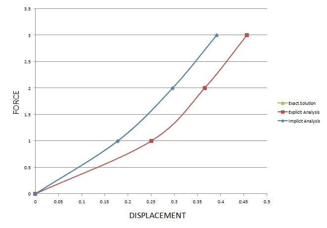
* Based on the results obtained from the above numerical calculation, a summary table is made and the results are plotted to compare the graphs.
SUMMARY TABLE :
| Step | Force | Displacement | ||
| Explicit Analysis | Implicit Analysis | Exact Solution | ||
| 0 | 0 | 0 | 0 | 0 |
| 1 | 1 | 0.25 | 0.178 | 0.178 |
| 2 | 2 | 0.365 | 0.296 | 0.296 |
| 3 | 3 | 0.456 | 0.391 | 0.391 |
GRAPH :
DISCUSSION :
- It is clear from both the graph and the table that the explicit analysis drifts from the exact solution. The drift from the exact
solution illustrates the lack of equilibrium between the internal and external forces. To correct for this problem an implicit analysis is required.
- The Newton-Raphson iterations correct the incremental steps so that they land on the exact solution according to the specified tolerance.
CONCLUSION :
Thus, the provided equation was solved using both Explicit and Implicit Methods and was compared with the actual result to evaulate the accuracy of each method.