Week - 2 - Explicit and Implicit Analysis

Week 2 Assignment - Explicit and Implicit Analysis

1. Write a detailed report about Implicit and explicit methods.

The Problems are expressed in mathematical partial differential equations. The equations are written in matric form as Linear and nonlinear.

Nonlinear problems fall into 3 categories.

Material Nonlinearity: deformations and strains are large (i.e., polymer materials)

Geometric Nonlinearity: strains are small, but rotations are large (i.e., thin structures)

Boundary Nonlinearity: Due to non-linearity of boundary conditions, (i.e., contact problems)

In linear problems, the partial differential equation is expressed in matrix equation as:

[K]{x} = {f}

and for non-linear static problems as:

[K(x)]{x} = {f}

For dynamic problems, the matrix equations can be written as:

[M]{x´´} + [C]{x´} + [K]{x} = {f}

where (.‘) represents the derivative.

Now coming to Implicit and explicit analysis:

Implicit analysis:

When the problem is nonlinear, the solution is obtained in several steps and the solution for the current step is based on the solution from the previous step. For large models, follows the iterative method, also known as the backward Euler integration scheme. These solutions are unconditionally stable and facilitate larger time steps. Despite this advantage, the implicit methods can be extremely time-consuming when solving dynamic and nonlinear problems.

Explicit analysis:

Explicit analysis objective is to solve for acceleration (or otherwise {x´´}). Once the accelerations are calculated at the nth step, the velocity (n+1/2 step) and displacement (n+1 step) are calculated accordingly. In these calculations, the arrangement is not unconditionally stable and thus smaller time steps are required. More accurately, the time step in an explicit finite element analysis must be less than the Courant time step (i.e., the time taken by a sound wave to travel transversely an element) while implicit analyses have no such limits.

Difference between Implicit and explicit analysis:

Explicit FEM is used when the state of a given system at a different timestep from the current time step to be calculated. In contrast, an implicit analysis finds a solution by solving an equation that includes both the current and future states of the given system. The implicit method requires additional computation and can be tough to implement.

2. Do the calculations in a spreadsheet, try to plot the graph and compare them?

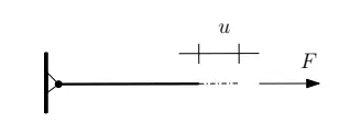
Considering the simple Bar tension case, as shown in fig 1

(fig. 1 )

and force in the nonlinear function of displacement equation:

F(u) = u3+9u2+4u (EQ 1)

and Stiffness of the bar K(u)= df/du = 3(u²) + 18(u) + 4 (EQ 2),

Clearly it is possible to plot a graph of force F, vs displacement u, by using equation (1).

Since Nonlinear relation between force and displacement is not known. And as stiffness variant is available a graph can be constructed numerically. One method is to use an incremental explicit load control scheme.

For example, 3 load variant increments ∆F=1 unit each are used to load the tension bar.

three equal load increments (or steps) of ∆F = 1 unit each are used to load the tension bar. The variables used are u for displacement, f for internal force in the bar, F for the external force applied to the bar, and k for stiffness. Incremental displacements or incremental externally applied forces are represented as ∆u or ∆F, respectively. Use is made of the relationship ∆F = k∆u.

and Let ∆F = k∆u. be (EQ 3)

The analysis proceeds as follows:

At Initial condition:

Step i1: u(0,0),

u0 = 0.0, ⇒ k(u0) = 1, ∆F = 1,

from eq 2, and eq 3

k(u) = 3(u²) + 18u + 4, = k(0) = 3(0²) + 18(0) + 4, = k(0) = 4

∆F = k∆u

1 = 4 ×∆u, = ∆u = 0.25

1st Iteration at u1 = u0 + ∆u1 = 0.25

after calualtating for u2, u3

u2 =0.36

u3= 0.46

Finally, from the three steps the following results are obtained.

Fext = ∆F + ∆F + ∆F = 3.0

for F(int)

from eq 1

F(u) = u3+9u2+4u

Fint 1 = (0.25³) + 9 × (0.25²) + 4 × (0.25) = 1.57

Fint 2 = (0.3651³) + 9 × (0.3651²) + 4 × (0.3651) = 2.708

Fint 3 = (0.4562³) + 9 × (0.4562²) + 4 × (0.4562) = 3.7928

Step i	∆Fi	∆ui	ui	F ext i	F int i	R= f int- f ext
1	1	0.25	0.25	1	1.57	0.57
2	1	0.11	0.36	2	2.70	0.70
3	1	0.09	0.45	3	3.79	0.79

Implicit analysis

An implicit analysis is the same as the explicit analysis, except that at the end of each step
Newton-Raphson iterations are used to enforce equilibrium before moving to the next step.
Basically, an incremental force is applied to advance the solution forward at the beginning
of a step. However, internal forces and external forces will not be in equilibrium unless the
stiffness is linear for the given step. Hence, in order to achieve equilibrium, corrections must
be made to the displacement.

This is accomplished by using Newton-Raphson iterations to minimize the residual, R(u) = fint − Fext. Expanding the residual as a Taylor series about

the current displacement u^j gives

R^j+1 = R^j(u^j) + dR(u^j)/du (δu^j+1) + ... = R^j + k(u^j)δu^j+1 + ...

By neglecting higher-order terms in the series, setting Rj+1 = 0 and solving for δuj+1 the following correction is obtained

δu^j+1 = −[k(u^j)]−1R^j

^Calculation:

^{Step 1, u(0,0)}

^{u0 = 0.0, ⇒ k(u0) = 4 (solving eq 2), ∆F = 1, ∆u0= 0.25}

^{u1= u0 + ∆u0 = 0.25}

F int1 = 1.5781 (by table above)

Fext = 1

R0 = fint1 − Fext1 = 0.578

as R0>0.01 , Newton-Raphson iterations are necessary.

u1 = u⁽⁰⁾

δu⁽¹⁾ = −[k(u₁⁽⁰⁾)]⁻¹R⁽⁰⁾

^{δu(1) = -0.066}

The updated value of u₁^{(1) = 0.184}

^{Check the residual again,}

^{R(1) = fint − Fext = 0.0469 (another Newton-Raphson iteration is necessary.)}

^{Calculate the new total correction to u1 = u₁(0)}

^{δu(2) = −[k(u₁(1))]−1R(1) = -0.0723}

^{The updated value of u₁(2) = 0.177}

^{checking residual again.}

after calculation

R2 = 0.0006 which is less than 0.01 therefore no need for further iterations.

same is found for both u2 = 0.29 , u3 = 0.39

The table follows:

Step i	∆Fi	∆ui	ui	F ext i	F int i	R= f int- f ext
1	1	0.25	0.177	1	1.0006	0.0006
2	1	0.11	0.29	2	2.00	0.0032
3	1	0.09	0.39	3	3.0	0.002

Graph:

Orange line: implicit

Blue Line: Explicit

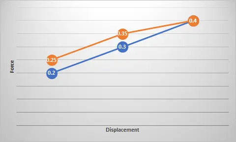
With a graph, it clearly shows that Implicit analysis which uses newton raphson iterative is more accurate than Explicit.