Week - 2 - Explicit and Implicit Analysis

The principal reason for using implicit solution methods, which are more complex to program and require more computational effort in each solution step, is to allow for large time-step sizes. A simple qualitative model will help to illustrate how this works. Let Q be a quantity whose value Qn+1 we want to compute at time t=(n+1)dt, in terms of its value at time t=ndt, i.e., Qn+1=Qn+dtS, where S is the rate of change in Q.

In an explicit numerical method S would be evaluated in terms of known quantities at the previous time step n. An implicit method, in contrast, would evaluate some or all of the terms in S in terms of unknown quantities at the new time step n+1. Since new quantities appear on both the left and right side of the Q-equation, it is said to be an implicit definition of the new n+1 values. Usually a matrix or iterative solution must be used to compute the new quantities.

Numerical stability has to do with the behavior of the solution as the time-step dt is increased. If the solution remains well behaved for arbitrarily large values of the time step, the method is said to be unconditionally stable. This situation never occurs with explicit methods, which are always conditionally stable. It is easy to see this by dividing the Q-equation by dt and then letting dt approach infinity. In this limit there are no n+1 terms remaining in the equation so no solution exists for Qn+1, indicating that there must be some limit on the size of the time step for there to be a solution.

In an implicit formulation, a solution for the unknowns at new time step n+1 may be obtained for any size time step. Of course, the solution for very large times may not be realistic unless the implicit formulation has been carefully constructed.

A typical iterative solution for Qn+1 is constructed by computing the k+1 iterate in terms of the kth iterate value, where the first iterate is taken to be equal to Qn. The equation for Qk+1 is often a Newton’s approximation (or similar approximation) having the form Qk+1=Qk+A(Qn-Qk+dtSk). In this expression A is a relaxation factor, and Sk is an approximation to S evaluated in terms of the kth iterate. If A is chosen properly, successive iterates will eventually converge to Qn+1.

The relaxation coefficient A must have the form A=1/(1+Cdt) in order to insure the proper limits at small and large values of dt. That is, at very small time-step sizes the explicit equation is recovered, while at very large time-step sizes the equation has a limiting value independent of dt. The quantity C must be a positive coefficient characterizing all the terms in the original equation (i.e., in S) that have been approximated implicitly. For example, if Q is a velocity component governed by a momentum equation with implicit viscous terms, then C would be proportional to the kinematic viscosity divided by the square of the grid size.

AIM :

To solve a non linear static problem by both explicit and implicit analysis.

Given Parameters :

A simple bar in tension as shown in Figure 1. Suppose that the force in the bar is a nonlinear function of the displacement F(u) = u³+9u²+4u

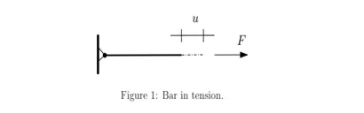
Three equal load increments (or steps) of ∆F = 1 unit each are used to load the tension bar. The variables used are u for displacement, f for internal force in the bar, F for external force applied to the bar and k for stiffness. Increemental displacements or incremental externally applied forces are represented as ∆u or ∆F, respectively. Use is made of the relationship ∆F = k∆u.

⇒k(u) = df/du = 3u²+18u+4

Explicit analysis :

Step 1 :

u₀ = 0, ⇒ k(u₀) = 4, ∆F = 1, ∆u₁ = ∆F/k(u₀) = 0.25, u₁ = u₀ + ∆u₁ = 0.25

Step 2 :

⇒ k(u₁) = 3*(0.25)² + 18*0.25+4 = 0.1875+4.5+4 = 8.6875, ∆F = 1, ∆u₂ = ∆F/k(u₁) = 0.1151, u₂ = u₁ + ∆u₂ = 0.3651

Step 3 :

⇒ k(u₂) = 3*(0.3651)²+18*0.3651+4 = 10.7178, ∆F = 1, ∆u₃ = ∆F/k(u₂) = 1/10.7178, u₃ = u₂+∆u₃= 0.4584

Finally, from the three steps the following results are obtained.

(F_int)₁ = u₁³+9u₁²+4*u₁ = 0.25³+9*0.25²+4*0.25 = 1.5781

(F_int)₂ = u₂³+9u₂²+4*u₂ = 0.3651³+9*0.0.3651²+4*0.3651 = 2.7087

(F_int)₃ = u₃³+9u₃²+4*u₃ = 0.4584³+9*0.4584²+4*0.4584 = 3.821

Step i	∆Fi	∆ui	ui	(Fext)i	(fint)i	fint − Fext = R
1	1	0.25	0.25	1	1.5781	0.5781
2	1	0.1151	0.3651	2	2.7087	0.7087
3	1	0.0933	0.4584	3	3.821	0.821

It is evident from the results that external and internal forces are NOT in equilibrium because
F_ext ≠ f_int.

Implicit Analysis :

An implicit analysis is the same as the explicit analysis, except that at the end of each step Newton-Raphson iterations are used to enforce equilibrium before moving to the next step. Basically, an incremental force is applied to advance the solution forward at the beginning of a step. However, internal forces and external forces will not be in equilibrium unless the stiffness is linear for the given step. Hence, in order to achieve equilibrium, corrections must be made to the displacement. This is accomplished by using Newton-Raphson iterations to minimize the residual, R_(u) = f_int − F_ext. Expanding the residual as a Taylor series about the current displacement u^j gives

R^j+1 = R^j(u^j) + dR(u^j)/du *δu^j+1 + ... = R^j + k(u^j)δu^j+1 + ...

By neglecting higher order terms in the series, setting R^j+1 = 0 and solving for δu^j+1 the

following correction is obtained

δu^j+1 = −[k(u^j)]⁻¹R^j

Notice that the iteration variable is j and it may take several iterations for the norm of the residual, ||R||, to be reduced below the chosen tolerance criteria (for the example below a tolerance of 10⁻² is chosen).

Step 1 :

u₀ = 0, ⇒ k(u₀) = 4, ∆F = 1, ∆u₁ = ∆F/k(u₀) = 0.25, u₁ = u₀ + ∆u₁ = 0.25

(F_int)₁ = u₁³+9u₁²+4*u₁ = 0.25³+9*0.25²+4*0.25 = 1.5781

R⁽⁰⁾ = f_int − F_ext = 1.5781 – 1 = 0.5781

||R⁽⁰⁾|| > 10⁻² ⇒ Newton-Raphson iterations is necessary.

the correction is δu⁽¹⁾ = −[k(u₁⁽⁰⁾)]⁻¹ * R⁽⁰⁾ = -[ 3*0.25²+18*0.25+4 ]^-1 * 0.5781 = -0.0665

⇒u₁¹=u₁⁰+∂u¹ = 0.25-0.0665 =0.1835

(F_int)₁ = u₁³+9u₁²+4*u₁ = 1.0432 > 10^-2 ⇒ Newton-Raphson iterations is necessary.

the correction is δu⁽²⁾ = −[k(u₁⁽¹⁾)]⁻¹ * R⁽¹⁾ = -[3*0.1835²+18*0.1835+4]^-1 * 0.0432 = -0.0058

u₁²=u₁⁰+u₁¹+∂u² = 0.25-0.0665-0.0058 =0.1777

(F_int)₁² = u₁³+9*u₁²+4*u₁ = 0.1777³ + 9*0.1777²+4*0.1777=1.0006

R⁽²⁾ = f_int − F_ext = 1.0006 – 1 = 0.0006 < 10⁻²

So, (F_int)₁ = 1.0006

Step 2 :

(F_int)₂ = u₂³+9u₂²+4*u₂ = 0.3651³+9*0.0.3651²+4*0.3651 = 2.7087

R⁽⁰⁾ = f_int − F_ext = 2.7087 – 2 = 0.7087

||R⁽⁰⁾|| > 10⁻² ⇒ Newton-Raphson iterations are necessary.

the correction is

δu⁽¹⁾ = −[k(u₂⁽⁰⁾)]⁻¹ * R⁽⁰⁾ = -[ 3*0.3651²+18*0.3651+4 ]^-1 * 0.5781 = -0.0646

u₂¹=u₂⁰+∂u¹ = 0.3651-0.0646 =0.3005

(F_int)₂¹ = u₂³+9*u₂²+4*u₂ = 0.3005³ + 9*0.3005²+4*0.3005=2.037

R⁽¹⁾ = f_int − F_ext = 2.037 – 2 = 0.037> 10^-2

the correction δu⁽²⁾ = −[k(u₂⁽¹⁾)]⁻¹ * R⁽¹⁾ = -[3*0.3005²+18*0.3005+4]^-1 * 0.037 = -0.0038

u₂²=u₂⁰+u₂¹+∂u² = 0.3651-0.0646-0.0038 =0.2967

(F_int)₁² = u₁³+9*u₁²+4*u₁ = 0.2967³ + 9*0.2967²+4*0.2967=2.0052

R⁽²⁾ = f_int − F_ext = 2.0052 – 2 = 0.0052 < 10⁻²

So, (F_int)₂ = 2.0052

Step 3 :

(F_int)₃ = u₃³+9u₃²+4*u₃ = 0.4584³+9*0.4584²+4*0.4584 = 3.821

R⁽⁰⁾ = f_int − F_ext = 3.821– 3 = 0.821

||R⁽⁰⁾|| > 10⁻² ⇒ Newton-Raphson iterations are necessary.

the correction is

δu⁽¹⁾ = −[k(u₃⁽⁰⁾)]⁻¹ * R⁽⁰⁾ = -[ 3*0.4584²+18*0.4584+4 ]^-1 * 0.821 = -0.0637

u₃¹=u₃⁰+∂u¹ = 0.4584-0.0637 =0.3947

(F_int)₃¹ = u₃³+9*u₃²+4*u₃ = 0.3947³ + 9*0.3947²+4*0.3947=3.0424

R⁽¹⁾ = f_int − F_ext = 3.0424 – 3 = 0.0424> 10^-2

the correction δu⁽²⁾ = −[k(u₃⁽¹⁾)]⁻¹ * R⁽¹⁾ = -[3*0.3947²+18*0.3947+4]^-1 * 0.0424 = -0.0037

u₂²=u₂⁰+u₂¹+∂u² = 0.4584-0.0637-0.0037 =0.3911

(F_int)₁² = u₁³+9*u₁²+4*u₁ = 0.3911³ + 9*0.3911²+4*0.3911=3.0009

R⁽³⁾ = f_int − F_ext = 3.0009 – 2 = 0.0009< 10⁻²

So, (F_int)₃ = 3.0009